음성 신호에서 스펙트로그램 해석
스펙트로그램 (또는 로그 크기 스펙트로그램)은 음성 신호의 효과적인 시각화이다. 스펙트로그램을 보면 고조파 구조 (harmonic structure), 시간적 사건 (temporal events), 음형대 (formants) 등 음성 신호의 가장 중요한 속성 중 다수를 볼 수 있다.
# Initialization
import matplotlib.pyplot as plt
from scipy.io import wavfile
import scipy
import scipy.fft
import numpy as np
import librosa
import librosa.display
import IPython.display as ipd

speechfile = 'sample.wav'
window_length_ms = 50
window_hop_ms = 3

def linearfilterbank(speclen, maxfreq_Hz, bandwidth_Hz=500):
    bandstep_Hz = bandwidth_Hz/2
    bands = int(maxfreq_Hz/bandstep_Hz)+1
    filterbank = np.zeros((speclen,bands))
    freqvec = np.arange(0,speclen,1)*maxfreq_Hz/speclen
    freq_idx = np.arange(-bandstep_Hz/2,maxfreq_Hz+bandstep_Hz/2,bandstep_Hz)
    for k in range(bands-1):
        if k>0:
            upslope = (freqvec-freq_idx[k])/(freq_idx[k+1]-freq_idx[k])
        else:
            upslope = 1 + 0*freqvec
        if k<bands-2:
            downslope = 1 - (freqvec-freq_idx[k+1])/(freq_idx[k+2]-freq_idx[k+1])
        else:
            downslope = 1 + 0*freqvec
        triangle = np.max([0*freqvec,np.min([upslope,downslope],axis=0)],axis=0)
        filterbank[:,k] = triangle

    reconstruct = np.matmul(np.diag(np.sum(filterbank**2+1e-12,axis=0)**-1),np.transpose(filterbank))

    return filterbank, reconstruct

def pow2dB(x): return 10.*np.log10(np.abs(x)+1e-12)
def dB2pow(x): return 10.**(x/10.)

speech, fs = librosa.load(speechfile)

# resample to 8kHz for better visualization
target_fs = 8000
speech = scipy.signal.resample(speech, len(speech)*target_fs//fs)
fs = target_fs

window_length = window_length_ms*fs//1000
spectrum_length = (window_length+2)//2
window_hop = window_hop_ms*fs//1000
windowing_function = np.sin(np.pi*np.arange(0.5, window_length, 1.)/window_length)

#melfilterbank, melreconstruct = helper_functions.melfilterbank(spectrum_length, fs/2, melbands=35)
filterbank, reconstruct = linearfilterbank(spectrum_length, fs/2, bandwidth_Hz=300)

Speech = librosa.stft(speech, n_fft=window_length, hop_length=window_hop)

frame_cnt = Speech.shape[1]
timebank, timereconstruct = linearfilterbank(frame_cnt, frame_cnt*window_hop_ms, bandwidth_Hz=120)

# envelope
SpeechEnvelope =  np.matmul(reconstruct.T,np.matmul(filterbank.T,np.abs(Speech)**2))**.5
FineFrequencyStructure = Speech/SpeechEnvelope
SpeechEnvelopeTime =  np.matmul(timereconstruct.T,np.matmul(timebank.T,np.abs(SpeechEnvelope.T)**2)).T**.5
FineTimeEnvelope = SpeechEnvelope/SpeechEnvelopeTime
Noise = np.random.randn(SpeechEnvelope.shape[0],SpeechEnvelope.shape[1])
SpeechFrequencyEnvelope = SpeechEnvelope*Noise
SpeechFineTime = FineTimeEnvelope*Noise
SpeechSmoothTime = SpeechEnvelopeTime*Noise

speechfrequencyenvelope = librosa.istft(SpeechFrequencyEnvelope, n_fft=window_length, hop_length=window_hop)
speechfinefrequency = librosa.istft(FineFrequencyStructure, n_fft=window_length, hop_length=window_hop)
speechsmoothtime = librosa.istft(SpeechSmoothTime, n_fft=window_length, hop_length=window_hop)
speechfinetime = librosa.istft(SpeechFineTime, n_fft=window_length, hop_length=window_hop)

fig, ax = plt.subplots(nrows=1, ncols=1, sharex=True, figsize=(8,3))
D = librosa.amplitude_to_db(np.abs(Speech), ref=np.max)
img = librosa.display.specshow(D, y_axis='linear', x_axis='time',sr=fs, hop_length=window_hop)
plt.title('Speech')
plt.xlabel('Time (s)')
plt.ylabel('Frequency (Hz)')
plt.show()

ipd.display(ipd.HTML("Original speech sound"))
ipd.display(ipd.Audio(speech,rate=fs))
#ipd.display(ipd.HTML("<hr>"))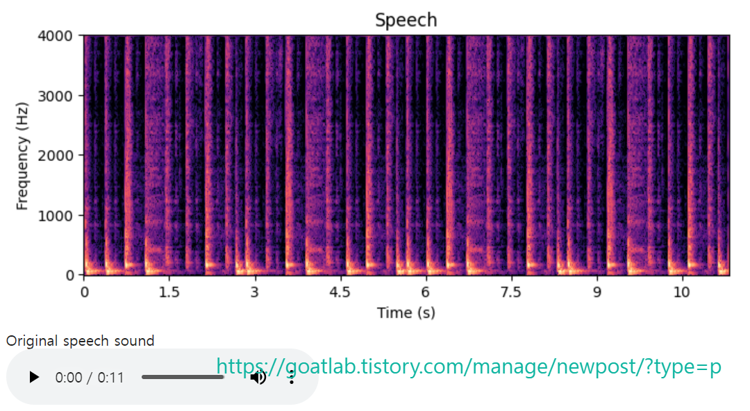
음성 신호의 가장 기본적인 특성은 음형대와 고조파 구조이다. 음형대는 주파수 축의 매크로 (macro) 레벨 모양에 해당하고, 하모닉 구조는 마이크로 (micro) 레벨 구조에 해당한다. 즉, 거시적 수준의 형상인 주파수 포락선 (envelope)을 추가하고 그 효과를 제거하면 고조파 구조를 얻게 된다.
fig, ax = plt.subplots(nrows=1, ncols=1, sharex=True, figsize=(8,3))
D = librosa.amplitude_to_db(np.abs(SpeechEnvelope), ref=np.max)
img = librosa.display.specshow(D, y_axis='linear', x_axis='time',sr=fs, hop_length=window_hop)
plt.title('Frequency Envelope')
plt.xlabel('Time (s)')
plt.ylabel('Frequency (Hz)')
plt.show()

ipd.display(ipd.HTML("White noise shaped by the frequency envelope (i.e. harmonic structure is removed)"))
ipd.display(ipd.Audio(speechfrequencyenvelope,rate=fs))
ipd.display(ipd.HTML("<hr>"))

fig, ax = plt.subplots(nrows=1, ncols=1, sharex=True, figsize=(8,3))
D = librosa.amplitude_to_db(np.abs(FineFrequencyStructure), ref=np.max)
img = librosa.display.specshow(D, y_axis='linear', x_axis='time',sr=fs, hop_length=window_hop)
plt.title('Harmonic Structure')
plt.xlabel('Time (s)')
plt.ylabel('Frequency (Hz)')
plt.show()

ipd.display(ipd.HTML("Harmonic structure"))
ipd.display(ipd.Audio(speechfinefrequency,rate=fs))
#ipd.display(ipd.HTML("<hr>"))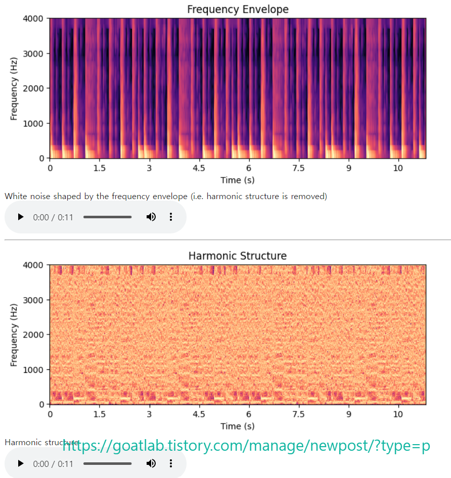
조화 구조에서 일정한 간격으로 간격을 두고 있는 수평선을 볼 수 있다. 가장 낮은 수평선은 기본 주파수에 해당한다. 그 위의 각 후속 라인은 기본 의 정수 배수에 배치된 고조파이다. 언어 생성 기관에서 기본 주파수는 성대 (vocal folds)의 진동에 의해 생성다. 부드러운 정현파 진동은 단일 주파수만 가지지만 성대 주름은 모든 진동에서 한 번 충돌하므로 파형의 날카로운 모서리에 해당하고 이는 차례로 주파수의 고조파 구조에 해당한다. 따라서, 날카롭고 밝고 긴장된 유성음은 눈에 띄는 화음 구조를 갖는 반면, 어둡고 부드러운 유성음은 눈에 보이는 화음 수가 적다. 화음 구조의 소리 예에서는 화음 구조에 해당하는 톱니 모양의 윙윙거리는 (buzzing) 소리를 들을 수 있다. 대조적으로, 고조파 구조가 백색 소음 (white noise)으로 대체된 포락 구조의 사운드 예에서는 여전히 텍스트 내용을 명확하게 식별할 수 있다.
그러나 포락선 구조의 스펙트로그램에는 여전히 두 가지 별개의 구성 요소가 있으며, 시간이 지남에 따라 빠르고 부드러운 변화로 표시된다. 빠른 변화는 파열음 (plosives)에 해당하는 반면, 느린 변화는 모음을 정의하는 성도 (vocal tract)의 변화에 의해 생성다. 주파수 포락선 추출과 유사한 접근 방식을 통해 시간에 따른 빠르고 부드러운 변화를 분리할 수 있다.
fig, ax = plt.subplots(nrows=1, ncols=1, sharex=True, figsize=(8,3))
D = librosa.amplitude_to_db(np.abs(SpeechEnvelopeTime), ref=np.max)
img = librosa.display.specshow(D, y_axis='linear', x_axis='time',sr=fs, hop_length=window_hop)
plt.title('Smoothed time')
plt.xlabel('Time (s)')
plt.ylabel('Frequency (Hz)')
plt.show()

ipd.display(ipd.HTML("White noise shaped by smooth time structure"))
ipd.display(ipd.Audio(speechsmoothtime,rate=fs))
ipd.display(ipd.HTML("<hr>"))

fig, ax = plt.subplots(nrows=1, ncols=1, sharex=True, figsize=(8,3))
D = librosa.amplitude_to_db(np.abs(FineTimeEnvelope), ref=np.max)
img = librosa.display.specshow(D, y_axis='linear', x_axis='time',sr=fs, hop_length=window_hop)
plt.xlabel('Time (s)')
plt.ylabel('Frequency (Hz)')
plt.title('Fine time structure')
plt.show()

ipd.display(ipd.HTML("White noise shaped by fine time structure"))
ipd.display(ipd.Audio(speechfinetime,rate=fs))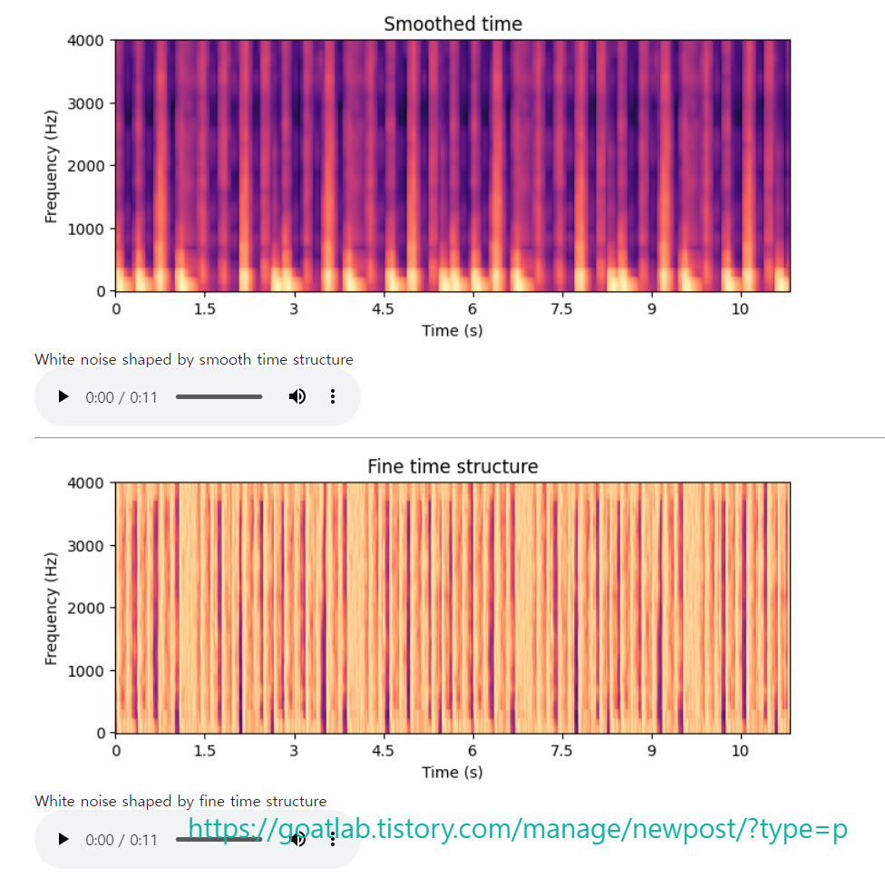
평활화된 시간 구조 및 평활화된 주파수 구조가 적용된 스펙트로그램 이미지에서는 시간에 따른 개별 이벤트에 해당하는 수직선이 제거된 것을 볼 수 있다. 일반적으로 정지 및 파열음에 해당한다. 이에 따라 미세 시간 구조의 스펙트로그램 이미지에서는 수직선만 보인다. 밝은 수직선 앞에는 종종 어두운 영역이 있다. 이는 공기 흐름이 방출되기 전에 완전히 멈추는 정지 자음이다. 따라서, 어두운 패치는 소리의 부재, 정지 및 release에 대한 다음의 밝은 선에 해당한다. 같은 유성 자음에는 유성음이 음소 전체에 걸쳐 계속될 수 있으므로 반드시 정지 부분이 있는 것은 아니다.
'Linguistic Intelligence > Audio Processing' 카테고리의 다른 글
| 영점 교차율 (Zero-crossing rate) (0) | 2024.04.24 |
|---|---|
| 자기 상관 관계 및 공분산 (0) | 2024.04.24 |
| 단시간 푸리에 변환 (STFT) (0) | 2024.04.23 |
| Sound Energy (0) | 2024.04.23 |
| 윈도우 기법 (Windowing) (0) | 2024.04.17 |


