728x90
반응형
SMALL
Multiple runs
# remember, this is here for running separate simulations in the same notebook
start_scope()
# Parameters
num_inputs = 100
input_rate = 10*Hz
weight = 0.1
# Range of time constants
tau_range = linspace(1, 10, 30)*ms
# Use this list to store output rates
output_rates = []
# Iterate over range of time constants
for tau in tau_range:
    # Construct the network each time
    P = PoissonGroup(num_inputs, rates=input_rate)
    eqs = '''
    dv/dt = -v/tau : 1
    '''
    G = NeuronGroup(1, eqs, threshold='v>1', reset='v=0', method='exact')
    S = Synapses(P, G, on_pre='v += weight')
    S.connect()
    M = SpikeMonitor(G)
    # Run it and store the output firing rate in the list
    run(1*second)
    output_rates.append(M.num_spikes/second)
# And plot it
plot(tau_range/ms, output_rates)
xlabel(r'$\tau$ (ms)')
ylabel('Firing rate (sp/s)');
start_scope()
num_inputs = 100
input_rate = 10*Hz
weight = 0.1
tau_range = linspace(1, 10, 30)*ms
output_rates = []
# Construct the network just once
P = PoissonGroup(num_inputs, rates=input_rate)
eqs = '''
dv/dt = -v/tau : 1
'''
G = NeuronGroup(1, eqs, threshold='v>1', reset='v=0', method='exact')
S = Synapses(P, G, on_pre='v += weight')
S.connect()
M = SpikeMonitor(G)
# Store the current state of the network
store()
for tau in tau_range:
    # Restore the original state of the network
    restore()
    # Run it with the new value of tau
    run(1*second)
    output_rates.append(M.num_spikes/second)
plot(tau_range/ms, output_rates)
xlabel(r'$\tau$ (ms)')
ylabel('Firing rate (sp/s)');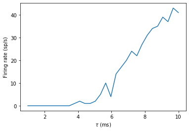
start_scope()
num_inputs = 100
input_rate = 10*Hz
weight = 0.1
tau_range = linspace(1, 10, 30)*ms
output_rates = []
# Construct the Poisson spikes just once
P = PoissonGroup(num_inputs, rates=input_rate)
MP = SpikeMonitor(P)
# We use a Network object because later on we don't
# want to include these objects
net = Network(P, MP)
net.run(1*second)
# And keep a copy of those spikes
spikes_i = MP.i
spikes_t = MP.t
# Now construct the network that we run each time
# SpikeGeneratorGroup gets the spikes that we created before
SGG = SpikeGeneratorGroup(num_inputs, spikes_i, spikes_t)
eqs = '''
dv/dt = -v/tau : 1
'''
G = NeuronGroup(1, eqs, threshold='v>1', reset='v=0', method='exact')
S = Synapses(SGG, G, on_pre='v += weight')
S.connect()
M = SpikeMonitor(G)
# Store the current state of the network
net = Network(SGG, G, S, M)
net.store()
for tau in tau_range:
    # Restore the original state of the network
    net.restore()
    # Run it with the new value of tau
    net.run(1*second)
    output_rates.append(M.num_spikes/second)
plot(tau_range/ms, output_rates)
xlabel(r'$\tau$ (ms)')
ylabel('Firing rate (sp/s)');
start_scope()
num_inputs = 100
input_rate = 10*Hz
weight = 0.1
tau_range = linspace(1, 10, 30)*ms
num_tau = len(tau_range)
P = PoissonGroup(num_inputs, rates=input_rate)
# We make tau a parameter of the group
eqs = '''
dv/dt = -v/tau : 1
tau : second
'''
# And we have num_tau output neurons, each with a different tau
G = NeuronGroup(num_tau, eqs, threshold='v>1', reset='v=0', method='exact')
G.tau = tau_range
S = Synapses(P, G, on_pre='v += weight')
S.connect()
M = SpikeMonitor(G)
# Now we can just run once with no loop
run(1*second)
output_rates = M.count/second # firing rate is count/duration
plot(tau_range/ms, output_rates)
xlabel(r'$\tau$ (ms)')
ylabel('Firing rate (sp/s)');
--> WARNING    "tau" is an internal variable of group "neurongroup", but also exists in the run namespace with the value 10. * msecond. The internal variable will be used. [brian2.groups.group.Group.resolve.resolution_conflict]
trains = M.spike_trains()
isi_mu = full(num_tau, nan)*second
isi_std = full(num_tau, nan)*second
for idx in range(num_tau):
    train = diff(trains[idx])
    if len(train)>1:
        isi_mu[idx] = mean(train)
        isi_std[idx] = std(train)
errorbar(tau_range/ms, isi_mu/ms, yerr=isi_std/ms)
xlabel(r'$\tau$ (ms)')
ylabel('Interspike interval (ms)');
Changing things during a run
start_scope()
# Parameters
area = 20000*umetre**2
Cm = 1*ufarad*cm**-2 * area
gl = 5e-5*siemens*cm**-2 * area
El = -65*mV
EK = -90*mV
ENa = 50*mV
g_na = 100*msiemens*cm**-2 * area
g_kd = 30*msiemens*cm**-2 * area
VT = -63*mV
# The model
eqs_HH = '''
dv/dt = (gl*(El-v) - g_na*(m*m*m)*h*(v-ENa) - g_kd*(n*n*n*n)*(v-EK) + I)/Cm : volt
dm/dt = 0.32*(mV**-1)*(13.*mV-v+VT)/
    (exp((13.*mV-v+VT)/(4.*mV))-1.)/ms*(1-m)-0.28*(mV**-1)*(v-VT-40.*mV)/
    (exp((v-VT-40.*mV)/(5.*mV))-1.)/ms*m : 1
dn/dt = 0.032*(mV**-1)*(15.*mV-v+VT)/
    (exp((15.*mV-v+VT)/(5.*mV))-1.)/ms*(1.-n)-.5*exp((10.*mV-v+VT)/(40.*mV))/ms*n : 1
dh/dt = 0.128*exp((17.*mV-v+VT)/(18.*mV))/ms*(1.-h)-4./(1+exp((40.*mV-v+VT)/(5.*mV)))/ms*h : 1
I : amp
'''
group = NeuronGroup(1, eqs_HH,
                    threshold='v > -40*mV',
                    refractory='v > -40*mV',
                    method='exponential_euler')
group.v = El
statemon = StateMonitor(group, 'v', record=True)
spikemon = SpikeMonitor(group, variables='v')
figure(figsize=(9, 4))
for l in range(5):
    group.I = rand()*50*nA
    run(10*ms)
    axvline(l*10, ls='--', c='k')
axhline(El/mV, ls='-', c='lightgray', lw=3)
plot(statemon.t/ms, statemon.v[0]/mV, '-b')
plot(spikemon.t/ms, spikemon.v/mV, 'ob')
xlabel('Time (ms)')
ylabel('v (mV)');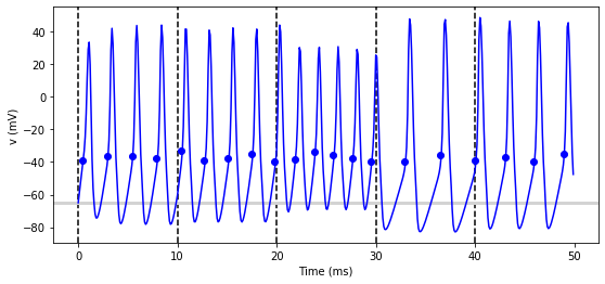
start_scope()
group = NeuronGroup(1, eqs_HH,
                    threshold='v > -40*mV',
                    refractory='v > -40*mV',
                    method='exponential_euler')
group.v = El
statemon = StateMonitor(group, 'v', record=True)
spikemon = SpikeMonitor(group, variables='v')
# we replace the loop with a run_regularly
group.run_regularly('I = rand()*50*nA', dt=10*ms)
run(50*ms)
figure(figsize=(9, 4))
# we keep the loop just to draw the vertical lines
for l in range(5):
    axvline(l*10, ls='--', c='k')
axhline(El/mV, ls='-', c='lightgray', lw=3)
plot(statemon.t/ms, statemon.v[0]/mV, '-b')
plot(spikemon.t/ms, spikemon.v/mV, 'ob')
xlabel('Time (ms)')
ylabel('v (mV)');
start_scope()
group = NeuronGroup(1, eqs_HH,
                    threshold='v > -40*mV',
                    refractory='v > -40*mV',
                    method='exponential_euler')
group.v = El
statemon = StateMonitor(group, 'v', record=True)
spikemon = SpikeMonitor(group, variables='v')
# we replace the loop with a network_operation
@network_operation(dt=10*ms)
def change_I():
    group.I = rand()*50*nA
run(50*ms)
figure(figsize=(9, 4))
for l in range(5):
    axvline(l*10, ls='--', c='k')
axhline(El/mV, ls='-', c='lightgray', lw=3)
plot(statemon.t/ms, statemon.v[0]/mV, '-b')
plot(spikemon.t/ms, spikemon.v/mV, 'ob')
xlabel('Time (ms)')
ylabel('v (mV)');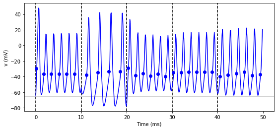
start_scope()
N = 3
eqs_HH_2 = '''
dv/dt = (gl*(El-v) - g_na*(m*m*m)*h*(v-ENa) - g_kd*(n*n*n*n)*(v-EK) + I)/C : volt
dm/dt = 0.32*(mV**-1)*(13.*mV-v+VT)/
    (exp((13.*mV-v+VT)/(4.*mV))-1.)/ms*(1-m)-0.28*(mV**-1)*(v-VT-40.*mV)/
    (exp((v-VT-40.*mV)/(5.*mV))-1.)/ms*m : 1
dn/dt = 0.032*(mV**-1)*(15.*mV-v+VT)/
    (exp((15.*mV-v+VT)/(5.*mV))-1.)/ms*(1.-n)-.5*exp((10.*mV-v+VT)/(40.*mV))/ms*n : 1
dh/dt = 0.128*exp((17.*mV-v+VT)/(18.*mV))/ms*(1.-h)-4./(1+exp((40.*mV-v+VT)/(5.*mV)))/ms*h : 1
I : amp
C : farad
'''
group = NeuronGroup(N, eqs_HH_2,
                    threshold='v > -40*mV',
                    refractory='v > -40*mV',
                    method='exponential_euler')
group.v = El
# initialise with some different capacitances
group.C = array([0.8, 1, 1.2])*ufarad*cm**-2*area
statemon = StateMonitor(group, variables=True, record=True)
# we go back to run_regularly
group.run_regularly('I = rand()*50*nA', dt=10*ms)
run(50*ms)
figure(figsize=(9, 4))
for l in range(5):
    axvline(l*10, ls='--', c='k')
axhline(El/mV, ls='-', c='lightgray', lw=3)
plot(statemon.t/ms, statemon.v.T/mV, '-')
xlabel('Time (ms)')
ylabel('v (mV)');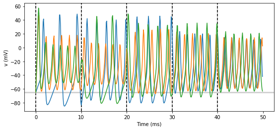
plot(statemon.t/ms, statemon.I.T/nA, '-')
xlabel('Time (ms)')
ylabel('I (nA)');
start_scope()
N = 3
eqs_HH_3 = '''
dv/dt = (gl*(El-v) - g_na*(m*m*m)*h*(v-ENa) - g_kd*(n*n*n*n)*(v-EK) + I)/C : volt
dm/dt = 0.32*(mV**-1)*(13.*mV-v+VT)/
    (exp((13.*mV-v+VT)/(4.*mV))-1.)/ms*(1-m)-0.28*(mV**-1)*(v-VT-40.*mV)/
    (exp((v-VT-40.*mV)/(5.*mV))-1.)/ms*m : 1
dn/dt = 0.032*(mV**-1)*(15.*mV-v+VT)/
    (exp((15.*mV-v+VT)/(5.*mV))-1.)/ms*(1.-n)-.5*exp((10.*mV-v+VT)/(40.*mV))/ms*n : 1
dh/dt = 0.128*exp((17.*mV-v+VT)/(18.*mV))/ms*(1.-h)-4./(1+exp((40.*mV-v+VT)/(5.*mV)))/ms*h : 1
I : amp (shared) # everything is the same except we've added this shared
C : farad
'''
group = NeuronGroup(N, eqs_HH_3,
                    threshold='v > -40*mV',
                    refractory='v > -40*mV',
                    method='exponential_euler')
group.v = El
group.C = array([0.8, 1, 1.2])*ufarad*cm**-2*area
statemon = StateMonitor(group, 'v', record=True)
group.run_regularly('I = rand()*50*nA', dt=10*ms)
run(50*ms)
figure(figsize=(9, 4))
for l in range(5):
    axvline(l*10, ls='--', c='k')
axhline(El/mV, ls='-', c='lightgray', lw=3)
plot(statemon.t/ms, statemon.v.T/mV, '-')
xlabel('Time (ms)')
ylabel('v (mV)');

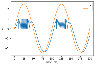
Adding input
start_scope()
A = 2.5
f = 10*Hz
tau = 5*ms
eqs = '''
dv/dt = (I-v)/tau : 1
I = A*sin(2*pi*f*t) : 1
'''
G = NeuronGroup(1, eqs, threshold='v>1', reset='v=0', method='euler')
M = StateMonitor(G, variables=True, record=True)
run(200*ms)
plot(M.t/ms, M.v[0], label='v')
plot(M.t/ms, M.I[0], label='I')
xlabel('Time (ms)')
ylabel('v')
legend(loc='best');

start_scope()
A = 2.5
f = 10*Hz
tau = 5*ms
# Create a TimedArray and set the equations to use it
t_recorded = arange(int(200*ms/defaultclock.dt))*defaultclock.dt
I_recorded = TimedArray(A*sin(2*pi*f*t_recorded), dt=defaultclock.dt)
eqs = '''
dv/dt = (I-v)/tau : 1
I = I_recorded(t) : 1
'''
G = NeuronGroup(1, eqs, threshold='v>1', reset='v=0', method='exact')
M = StateMonitor(G, variables=True, record=True)
run(200*ms)
plot(M.t/ms, M.v[0], label='v')
plot(M.t/ms, M.I[0], label='I')
xlabel('Time (ms)')
ylabel('v')
legend(loc='best');
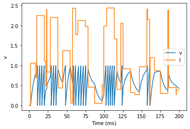
start_scope()
A = 2.5
f = 10*Hz
tau = 5*ms
# Let's create an array that couldn't be
# reproduced with a formula
num_samples = int(200*ms/defaultclock.dt)
I_arr = zeros(num_samples)
for _ in range(100):
    a = randint(num_samples)
    I_arr[a:a+100] = rand()
I_recorded = TimedArray(A*I_arr, dt=defaultclock.dt)
eqs = '''
dv/dt = (I-v)/tau : 1
I = I_recorded(t) : 1
'''
G = NeuronGroup(1, eqs, threshold='v>1', reset='v=0', method='exact')
M = StateMonitor(G, variables=True, record=True)
run(200*ms)
plot(M.t/ms, M.v[0], label='v')
plot(M.t/ms, M.I[0], label='I')
xlabel('Time (ms)')
ylabel('v')
legend(loc='best');
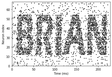
start_scope()
from matplotlib.image import imread
img = (1-imread('brian.png'))[::-1, :, 0].T
num_samples, N = img.shape
ta = TimedArray(img, dt=1*ms) # 228
A = 1.5
tau = 2*ms
eqs = '''
dv/dt = (A*ta(t, i)-v)/tau+0.8*xi*tau**-0.5 : 1
'''
G = NeuronGroup(N, eqs, threshold='v>1', reset='v=0', method='euler')
M = SpikeMonitor(G)
run(num_samples*ms)
plot(M.t/ms, M.i, '.k', ms=3)
xlim(0, num_samples)
ylim(0, N)
xlabel('Time (ms)')
ylabel('Neuron index');
https://brian2.readthedocs.io/en/stable/resources/tutorials/3-intro-to-brian-simulations.html
Introduction to Brian part 3: Simulations — Brian 2 2.5.0.3 documentation
If you haven’t yet read parts 1 and 2 on Neurons and Synapses, go read them first. This tutorial is about managing the slightly more complicated tasks that crop up in research problems, rather than the toy examples we’ve been looking at so far. So we c
brian2.readthedocs.io
728x90
반응형
LIST
'Natural Intelligence > Computational Neuroscience' 카테고리의 다른 글
| [Computational Neuroscience] 신경의 흥분성 (Nerve Excitability) (0) | 2022.09.20 |
|---|---|
| [Brian] Example : Spiking model (0) | 2022.02.14 |
| [Brian] Introduction to Brian part 2 : Synapses (0) | 2022.02.14 |
| [Brian] Introduction to Brian part 1 : Neurons (0) | 2022.02.11 |
| Brian 2 (0) | 2022.02.11 |


