728x90
반응형
SMALL
The simplest Synapse
start_scope()

eqs = '''
dv/dt = (I-v)/tau : 1
I : 1
tau : second
'''
G = NeuronGroup(2, eqs, threshold='v>1', reset='v = 0', method='exact')
G.I = [2, 0]
G.tau = [10, 100]*ms

# Comment these two lines out to see what happens without Synapses
S = Synapses(G, G, on_pre='v_post += 0.2')
S.connect(i=0, j=1)

M = StateMonitor(G, 'v', record=True)

run(100*ms)

plot(M.t/ms, M.v[0], label='Neuron 0')
plot(M.t/ms, M.v[1], label='Neuron 1')
xlabel('Time (ms)')
ylabel('v')
legend();
--> <matplotlib.legend.Legend at 0x7fdccb8773d0>
Adding a weight
start_scope()

eqs = '''
dv/dt = (I-v)/tau : 1
I : 1
tau : second
'''
G = NeuronGroup(3, eqs, threshold='v>1', reset='v = 0', method='exact')
G.I = [2, 0, 0]
G.tau = [10, 100, 100]*ms

# Comment these two lines out to see what happens without Synapses
S = Synapses(G, G, 'w : 1', on_pre='v_post += w')
S.connect(i=0, j=[1, 2])
S.w = 'j*0.2'

M = StateMonitor(G, 'v', record=True)

run(50*ms)

plot(M.t/ms, M.v[0], label='Neuron 0')
plot(M.t/ms, M.v[1], label='Neuron 1')
plot(M.t/ms, M.v[2], label='Neuron 2')
xlabel('Time (ms)')
ylabel('v')
legend();
--> <matplotlib.legend.Legend at 0x7fdccb7f2750>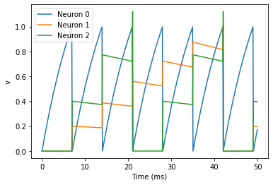
Introducing a delay
start_scope()

eqs = '''
dv/dt = (I-v)/tau : 1
I : 1
tau : second
'''
G = NeuronGroup(3, eqs, threshold='v>1', reset='v = 0', method='exact')
G.I = [2, 0, 0]
G.tau = [10, 100, 100]*ms

S = Synapses(G, G, 'w : 1', on_pre='v_post += w')
S.connect(i=0, j=[1, 2])
S.w = 'j*0.2'
S.delay = 'j*2*ms'

M = StateMonitor(G, 'v', record=True)

run(50*ms)

plot(M.t/ms, M.v[0], label='Neuron 0')
plot(M.t/ms, M.v[1], label='Neuron 1')
plot(M.t/ms, M.v[2], label='Neuron 2')
xlabel('Time (ms)')
ylabel('v')
legend();
--> <matplotlib.legend.Legend at 0x7fdccb7f2290>
More complex connectivity
start_scope()

N = 10
G = NeuronGroup(N, 'v:1')
S = Synapses(G, G)
S.connect(condition='i!=j', p=0.2)

def visualise_connectivity(S):
    Ns = len(S.source)
    Nt = len(S.target)
    figure(figsize=(10, 4))
    subplot(121)
    plot(zeros(Ns), arange(Ns), 'ok', ms=10)
    plot(ones(Nt), arange(Nt), 'ok', ms=10)
    for i, j in zip(S.i, S.j):
        plot([0, 1], [i, j], '-k')
    xticks([0, 1], ['Source', 'Target'])
    ylabel('Neuron index')
    xlim(-0.1, 1.1)
    ylim(-1, max(Ns, Nt))
    subplot(122)
    plot(S.i, S.j, 'ok')
    xlim(-1, Ns)
    ylim(-1, Nt)
    xlabel('Source neuron index')
    ylabel('Target neuron index')

visualise_connectivity(S)
start_scope()
N = 10
G = NeuronGroup(N, 'v:1')
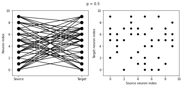
for p in [0.1, 0.5, 1.0]:
S = Synapses(G, G)
S.connect(condition='i!=j', p=p)
visualise_connectivity(S)
suptitle('p = '+str(p));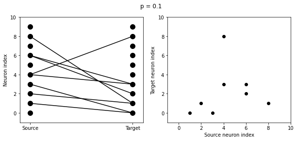

start_scope()

N = 10
G = NeuronGroup(N, 'v:1')

S = Synapses(G, G)
S.connect(condition='abs(i-j)<4 and i!=j')
visualise_connectivity(S)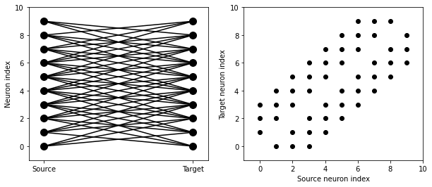
start_scope()

N = 10
G = NeuronGroup(N, 'v:1')

S = Synapses(G, G)
S.connect(j='k for k in range(i-3, i+4) if i!=k', skip_if_invalid=True)
visualise_connectivity(S)
start_scope()

N = 10
G = NeuronGroup(N, 'v:1')

S = Synapses(G, G)
S.connect(j='i')
visualise_connectivity(S)
start_scope()

N = 30
neuron_spacing = 50*umetre
width = N/4.0*neuron_spacing

# Neuron has one variable x, its position
G = NeuronGroup(N, 'x : metre')
G.x = 'i*neuron_spacing'

# All synapses are connected (excluding self-connections)
S = Synapses(G, G, 'w : 1')
S.connect(condition='i!=j')
# Weight varies with distance
S.w = 'exp(-(x_pre-x_post)**2/(2*width**2))'

scatter(S.x_pre/um, S.x_post/um, S.w*20)
xlabel('Source neuron position (um)')
ylabel('Target neuron position (um)');
--> Text(0, 0.5, 'Target neuron position (um)')
More complex synapse models : STDP
tau_pre = tau_post = 20*ms
A_pre = 0.01
A_post = -A_pre*1.05
delta_t = linspace(-50, 50, 100)*ms
W = where(delta_t>0, A_pre*exp(-delta_t/tau_pre), A_post*exp(delta_t/tau_post))
plot(delta_t/ms, W)
xlabel(r'$\Delta t$ (ms)')
ylabel('W')
axhline(0, ls='-', c='k');
--> <matplotlib.lines.Line2D at 0x7fdccb5acdd0>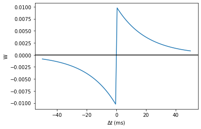
start_scope()

taupre = taupost = 20*ms
wmax = 0.01
Apre = 0.01
Apost = -Apre*taupre/taupost*1.05

G = NeuronGroup(2, 'v:1', threshold='t>(1+i)*10*ms', refractory=100*ms)

S = Synapses(G, G,
             '''
             w : 1
             dapre/dt = -apre/taupre : 1 (clock-driven)
             dapost/dt = -apost/taupost : 1 (clock-driven)
             ''',
             on_pre='''
             v_post += w
             apre += Apre
             w = clip(w+apost, 0, wmax)
             ''',
             on_post='''
             apost += Apost
             w = clip(w+apre, 0, wmax)
             ''', method='linear')
S.connect(i=0, j=1)
M = StateMonitor(S, ['w', 'apre', 'apost'], record=True)

run(30*ms)

figure(figsize=(4, 8))
subplot(211)
plot(M.t/ms, M.apre[0], label='apre')
plot(M.t/ms, M.apost[0], label='apost')
legend()
subplot(212)
plot(M.t/ms, M.w[0], label='w')
legend(loc='best')
xlabel('Time (ms)');
--> Text(0.5, 0, 'Time (ms)')
start_scope()

taupre = taupost = 20*ms
Apre = 0.01
Apost = -Apre*taupre/taupost*1.05
tmax = 50*ms
N = 100

# Presynaptic neurons G spike at times from 0 to tmax
# Postsynaptic neurons G spike at times from tmax to 0
# So difference in spike times will vary from -tmax to +tmax
G = NeuronGroup(N, 'tspike:second', threshold='t>tspike', refractory=100*ms)
H = NeuronGroup(N, 'tspike:second', threshold='t>tspike', refractory=100*ms)
G.tspike = 'i*tmax/(N-1)'
H.tspike = '(N-1-i)*tmax/(N-1)'

S = Synapses(G, H,
             '''
             w : 1
             dapre/dt = -apre/taupre : 1 (event-driven)
             dapost/dt = -apost/taupost : 1 (event-driven)
             ''',
             on_pre='''
             apre += Apre
             w = w+apost
             ''',
             on_post='''
             apost += Apost
             w = w+apre
             ''')
S.connect(j='i')

run(tmax+1*ms)

plot((H.tspike-G.tspike)/ms, S.w)
xlabel(r'$\Delta t$ (ms)')
ylabel(r'$\Delta w$')
axhline(0, ls='-', c='k');
--> <matplotlib.lines.Line2D at 0x7fdcc8ae8890>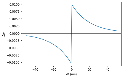
https://brian2.readthedocs.io/en/stable/resources/tutorials/2-intro-to-brian-synapses.html
Introduction to Brian part 2: Synapses — Brian 2 2.5.0.3 documentation
If you haven’t yet read part 1: Neurons, go read that now. As before we start by importing the Brian package and setting up matplotlib for IPython: The simplest Synapse Once you have some neurons, the next step is to connect them up via synapses. We’ll
brian2.readthedocs.io
728x90
반응형
LIST
'Natural Intelligence > Computational Neuroscience' 카테고리의 다른 글
| [Brian] Example : Spiking model (0) | 2022.02.14 |
|---|---|
| [Brian] Introduction to Brian part 3 : Simulations (0) | 2022.02.14 |
| [Brian] Introduction to Brian part 1 : Neurons (0) | 2022.02.11 |
| Brian 2 (0) | 2022.02.11 |
| [Computational Neuroscience] Molecular Dynamics : Periodic Boundary Conditions (0) | 2022.01.19 |


