Multiclass Classification Error Metrics
둘 이상의 결과를 예측하려면 둘 이상의 출력 뉴런이 필요하다. 하나의 뉴런이 두 가지 결과를 예측할 수 있기 때문에 출력 뉴런이 두 개인 신경망은 다소 드물다. 결과가 세 개 이상이면 출력 뉴런이 세 개 이상 필요하다.
import pandas as pd
from scipy.stats import zscore

# Read the dataset
df = pd.read_csv("https://data.heatonresearch.com/data/t81-558/jh-simple-dataset.csv", na_values=['NA', '?'])

# Generate dummies for job
df = pd.concat([df, pd.get_dummies(df['job'], prefix="job")], axis=1)
df.drop('job', axis=1, inplace=True)

# Generate dummies for area
df = pd.concat([df, pd.get_dummies(df['area'], prefix="area")], axis=1)
df.drop('area', axis=1, inplace=True)

# Missing values for income
med = df['income'].median()
df['income'] = df['income'].fillna(med)

# Standardize ranges
df['income'] = zscore(df['income'])
df['aspect'] = zscore(df['aspect'])
df['save_rate'] = zscore(df['save_rate'])
df['age'] = zscore(df['age'])
df['subscriptions'] = zscore(df['subscriptions'])

# Convert to numpy - Classification
x_columns = df.columns.drop('product').drop('id')
x = df[x_columns].values
dummies = pd.get_dummies(df['product'])  # Classification
products = dummies.columns
y = dummies.values
import numpy as np
import tensorflow.keras
from tensorflow.keras.models import Sequential
from tensorflow.keras.layers import Dense, Activation
from tensorflow.keras.callbacks import EarlyStopping
from sklearn.model_selection import train_test_split
# Split into train/test
x_train, x_test, y_train, y_test = train_test_split(
x, y, test_size=0.25, random_state=42)
model = Sequential()
model.add(Dense(100, input_dim=x.shape[1], activation='relu',
kernel_initializer='random_normal'))
model.add(Dense(50, activation='relu', kernel_initializer='random_normal'))
model.add(Dense(25, activation='relu', kernel_initializer='random_normal'))
model.add(Dense(y.shape[1], activation='softmax', kernel_initializer='random_normal'))
model.compile(loss='categorical_crossentropy',
optimizer=tensorflow.keras.optimizers.Adam(),
metrics=['accuracy'])
monitor = EarlyStopping(monitor='val_loss', min_delta=1e-3, patience=5,
verbose=1, mode='auto', restore_best_weights=True)
model.fit(x_train, y_train, validation_data=(x_test, y_test),
callbacks=[monitor], verbose=2, epochs=1000)
분류 정확도 계산
정확도는 신경망이 목표 클래스를 정확하게 예측한 행의 수이다. 정확도는 분류에만 사용되며 회귀에는 사용되지 않는다.

여기서 c는 정답 수이고 N은 평가된 집합 (학습 또는 검증)의 크기이다. 정확도가 높을수록 좋다. 기본적으로 Keras는 각 클래스에 대한 백분율 확률을 반환한다. 이러한 예측 확률을 argmax로 예측한 실제 홍채로 변경할 수 있다.
from sklearn import metrics

pred = model.predict(x_test)
pred = np.argmax(pred, axis=1)

y_compare = np.argmax(y_test, axis=1)
score = metrics.accuracy_score(y_compare, pred)
print("Accuracy score: {}".format(score))
분류 로그 손실 계산
정확도는 부분 점수가 없는 시험과 같다. 그러나 신경망은 각 대상 클래스의 확률을 예측할 수 있다. 신경망은 가능성이 더 높은 예측에 높은 확률을 부여한다. 로그 손실은 오답에 대한 신뢰도에 불이익을 주는 오류 메트릭이다. 로그 손실 값이 낮을수록 좋다.
from IPython.display import display
import numpy as np
from sklearn import metrics

# Don't display numpy in scientific notation
np.set_printoptions(precision=4)
np.set_printoptions(suppress=True)

# Generate predictions
pred = model.predict(x_test)
print("Numpy array of predictions")
display(pred[0:5])
print("As percent probability")
print(pred[0] * 100)
score = metrics.log_loss(y_test, pred)
print("Log loss score: {}".format(score))

# raw probabilities to chosen class (highest probability)
pred = np.argmax(pred, axis=1)
로그 손실은 다음과 같이 계산된다.

이 방정식은 두 가지 결과가 있는 분류의 목적 함수로만 사용해야 한다. 변수 y-hat은 신경망의 예측이고 변수 y는 알려진 정답이다. 이 경우 y는 항상 0 또는 1이 된다. 훈련 데이터에는 확률이 없다. 신경망은 이를 한 클래스(1) 또는 다른 클래스(0)로 분류한다.
변수 N은 훈련 세트의 요소 수와 테스트의 문제 수를 나타낸다. 이 과정은 평균을 구하기 위한 관례이므로 N으로 나눈다. 또한, 로그 함수는 0에서 1까지의 영역에서 항상 음수이기 때문에 방정식을 음수로 시작한다. 이 음수는 훈련의 점수를 최소화할 수 있는 양수이다.
두 항이 더하기(+)로 구분되어 있는 것을 볼 수 있다. 각각 로그 함수가 포함되어 있다. y는 0 또는 1이 될 것이므로 이 두 항 중 하나는 0으로 상쇄된다. y가 0이면 첫 번째 항이 0으로 줄어들고, y가 1이면 두 번째 항이 0이 된다.
두 등급 예측의 첫 번째 등급에 대한 예측이 Y-모양이면 두 번째 등급에 대한 예측은 1에서 Y-모양을 뺀 값이다. 즉, A 등급에 대한 예측이 70% (0.7)라면 B 등급에 대한 예측은 30% (0.3)가 된다. 점수는 올바른 클래스에 대한 예측 로그만큼 증가한다. 신경망이 클래스 A에 대해 1.0을 예측했고 정답이 A였다면 점수는 로그(1)만큼 증가하여 0이 된다. 로그 손실의 경우 낮은 점수를 추구하므로 정답은 0이 된다.
정답에 낮은 신뢰도를 부여하는 것이 점수에 가장 큰 영향을 미친다. 로그(0)은 음의 무한대이므로 일반적으로 최소값을 부과다. 물론 위의 로그 값은 단일 훈련 세트 요소에 대한 것이다. 전체 훈련 세트에 대한 로그 값의 평균을 구한다.
로그 함수는 오답에 불이익을 주는 데 유용하다. 다음 코드는 로그 함수의 유용성을 보여준다.
import matplotlib.pyplot as plt
from matplotlib.pyplot import figure, show
from numpy import arange, sin, pi

# t = arange(1e-5, 5.0, 0.00001)
# t = arange(1.0, 5.0, 0.00001) # computer scientists
t = arange(0.0, 1.0, 0.00001) # data scientists

fig = figure(1, figsize=(12, 10))
ax1 = fig.add_subplot(211)
ax1.plot(t, np.log(t))
ax1.grid(True)
ax1.set_ylim((-8, 1.5))
ax1.set_xlim((-0.1, 2))
ax1.set_xlabel('x')
ax1.set_ylabel('y')
ax1.set_title('log(x)')
show()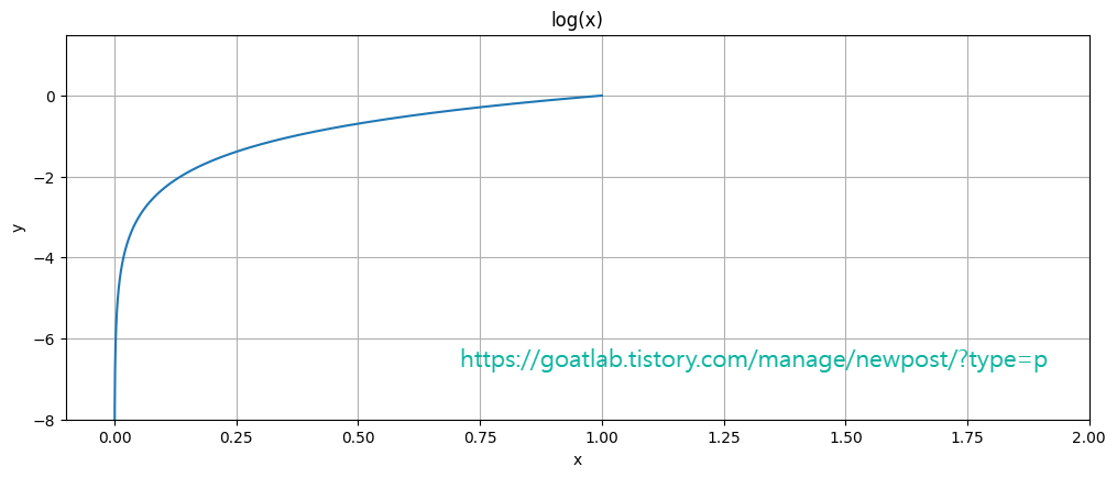
'DNN with Keras > Training for Tabular Data' 카테고리의 다른 글
| ROC 및 AUC를 사용한 다중클래스 분류 (0) | 2023.11.07 |
|---|---|
| 신경망을 위한 X 및 Y 생성 (0) | 2023.11.07 |
| 딥러닝을 위한 특징 벡터 인코딩 (0) | 2023.11.07 |


