728x90
반응형
SMALL
비선형 SVM 분류
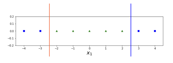
데이터가 선형적으로 분류가 안되는 경우에 사용한다. 그림을 보면, 빨강색과 파란색 직선 둘 다 완벽한 분류기가 되지 않았다. 이와 같이 실생활에서는 선형적으로 분류할 수 없는 데이터가 많다. 따라서, 데이터를 분류하기 쉽게 (선형적으로 분류 가능하도록) 만드는 작업을 진행해야 한다.
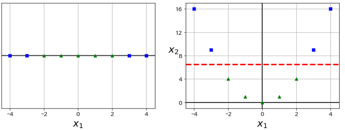
간단한 방법인 X1과 X1의 제곱 값을 X2에 대입한다. 빨강색 선과 같이 분명하게 나누어 진다. 이와 같이 Scikitlearn에서는 PolynomialFeatures 방식을 제공한다.
example
|
import numpy as np
from sklearn import datasets
from sklearn.pipeline import Pipeline
from sklearn.preprocessing import StandardScaler
from sklearn.svm import LinearSVC
from sklearn.svm import SVC

import matplotlib.pyplot as plt
from sklearn.datasets import make_moons
from sklearn.pipeline import Pipeline
from sklearn.preprocessing import PolynomialFeatures
%matplotlib inline

X, y = make_moons(n_samples=100, noise=0.15, random_state=42)

def plot_dataset(X, y, axes):
    plt.plot(X[y==0, 0], X[y==0, 1], "bs")
    plt.plot(X[y==1, 0], X[y==1, 1], "g^")
    plt.axis(axes)
    plt.grid(True, which="both")
    plt.xlabel("$x_1$")
    plt.ylabel("$x_2$")

plt.scatter(X[:,0], X[:,1], marker='o', c=y, s=100, edgecolor="k", linewidth=2)
plt.show()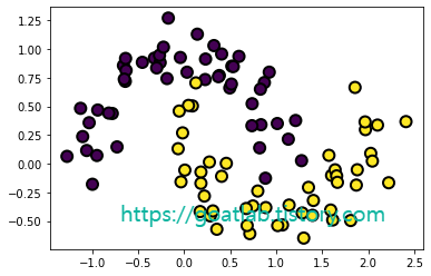
polynomial_svm_clf = Pipeline([
    ('poly_features', PolynomialFeatures(degree = 3)),
    ('scaler', StandardScaler()),
    ("svm_clf", LinearSVC(C = 10, loss = "hinge")),
])

polynomial_svm_clf.fit(X, y)
def plot_prediction(clf, axes):
x0s = np.linspace(axes[0], axes[1], 100)
x1s = np.linspace(axes[2], axes[3], 100)
x0, x1 = np.meshgrid(x0s, x1s)
X = np.c_[x0.ravel(), x1.ravel()]
y_pred = clf.predict(X).reshape(x0.shape)
y_decision = clf.decision_function(X).reshape(x0.shape)
plt.contourf(x0, x1, y_pred, cmap=plt.cm.brg, alpha=0.2)
plt.contourf(x0, x1, y_decision, cmap=plt.cm.brg, alpha=0.1)
plot_prediction(polynomial_svm_clf, [-1.5, 2.5, -1.5, 1.5])
plot_dataset(X, y, [-1.5, 2.5, -1.5, 1.5])
plt.show()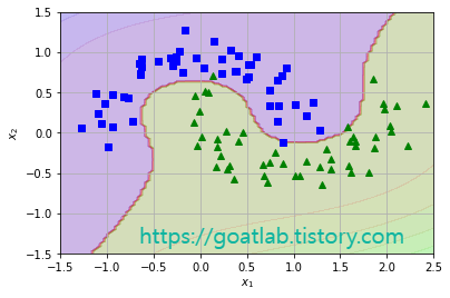
다항식 커널
다항식 특성을 추가하는 것은 간단하지만, 낮은 차수의 다항식은 매우 복잡한 데이터셋을 잘 표현하지 못하고 높은 차수의 다항식은 굉장히 많은 특성을 추가해야 해서 모델 수행이 느리다. 커널 트릭은 실제 특성을 추가하지 않고도 수학적 기교를 이용하여 다항식 특성을 많이 추가한 것과 같은 결과를 얻을 수 있다. Scikit-learn에서는 SVC 클래스에 커널 트릭이 구현되어 있으며, 이것을 Parameter로 설정한다.
from sklearn.svm import SVC
poly_kernel_svm_clf = Pipeline([
    ("scaler", StandardScaler()),
    ("svm_clf", SVC(kernel="poly", degree=3, coef0=1, C=5))
])

poly_kernel_svm_clf.fit(X, y)
from sklearn.svm import SVC
poly100_kernel_svm_clf = Pipeline([
("scaler", StandardScaler()),
("svm_clf", SVC(kernel="poly", degree=10, coef0=100, C=5))
])
poly100_kernel_svm_clf.fit(X, y)plt.figure(figsize=(11, 4))
plt.subplot(121)
plot_prediction(poly_kernel_svm_clf, [-1.5, 2.5, -1.5, 1.5])
plot_dataset(X, y, [-1.5, 2.5, -1.5, 1.5])
plt.title(r"$d=3, r=1, C=5$", fontsize=18)
plt.subplot(122)
plot_prediction(poly100_kernel_svm_clf, [-1.5, 2.5, -1.5, 1.5])
plot_dataset(X, y, [-1.5, 2.5, -1.5, 1.5])
plt.title(r"$d=10, r=100, C=5$", fontsize=18)
plt.show()
from sklearn.svm import SVC
poly_kernel_svm_clf = Pipeline([
    ("scaler", StandardScaler()),
    ("svm_clf", SVC(kernel="linear", degree=3, coef0=1, C=5))
])

poly_kernel_svm_clf.fit(X, y)
Kernel Trick 알고리즘의 수식

plt.figure(figsize=(11, 4))
plt.subplot(121)
plot_prediction(poly_kernel_svm_clf, [-1.5, 2.5, -1.5, 1.5])
plot_dataset(X, y, [-1.5, 2.5, -1.5, 1.5])
plt.title(r"$d=3, r=1, C=5$", fontsize=18)
728x90
반응형
LIST
'Learning-driven Methodology > ML (Machine Learning)' 카테고리의 다른 글
| [Machine Learning] LightGBM (0) | 2022.10.04 |
|---|---|
| [Machine Learning] SVM 회귀 (0) | 2022.09.30 |
| [LightGBM] 매개변수 조정 (Parameters Tuning) (2) (0) | 2022.07.04 |
| [LightGBM] 매개변수 조정 (Parameters Tuning) (1) (0) | 2022.06.28 |
| [LightGBM] Features (2) (0) | 2022.06.28 |


