스펙트로그램 (Spectrogram)
스펙트로그램은 음성 신호의 많은 관련 특징을 효과적으로 시각화한다는 점에서 음성을 표현하는 데 유용하다. 특히, 시간 경과에 따른 이벤트, 기본 주파수의 변화, 스펙트럼 포락선 (spectral envelope)의 일부 특징을 관찰할 수 있다. 하지만 단점도 있다. 스펙트럼은 원하는 정보의 양에 비해 많은 수의 계수 (coefficients)를 가지고 있기 때문에 계수 수 측면에서 특별히 효율적인 표현이 아니다. 일반적으로 포먼트 (formant)의 위치와 진폭에 대한 정보를 원하는데, 이는 몇 개의 계수로 표현할 수 있다. 마찬가지로 기본 주파수는 하나의 정보에 불과하지만 수많은 주파수 성분에 숨겨져 있다.
캡스트럼 (Cepstrum)
예를 들어, 음성 신호의 많은 중심 속성은 로그 스펙트럼에서 구조로 명확하게 볼 수 있다. 예를 들어, F0 주파수에서 포락선은 부드러운 매크로 구조이고 기본 주파수는 고조파 빗 (harmonic comb) 구조이다. 두 가지 유형의 구조는 모두 시간-주파수 변환 (time-frequency transform)으로 쉽게 분석할 수 있다. 특히, 로그 스펙트럼에서 구조를 볼 수 있으므로 로그 스펙트럼의 이산 푸리에 변환 또는 이산 코사인 변환 (discrete cosine transform)을 사용해야 한다. 따라서, 원래 시간 신호에 두 개의 시간-주파수 변환을 적용하되 그 사이에 비선형 연산인 절대값의 로그를 적용하는 것이다. 알고리즘은 다음과 같다.
|
두 번째 시간-주파수 변환 후의 출력은 스펙트럼의 역변환이기 때문에 캡스트럼이라고 한다. 마찬가지로, 캡스트럼의 x축은 주파수에 대응하기 때문에 quefrency라고 한다. 캡스트럼은 두 개의 연속적인 시간-주파수 변환의 결과이므로, quefrency의 단위는 초가 된다.
import matplotlib.pyplot as plt
from scipy.io import wavfile
import scipy
import scipy.fft
import numpy as np

np.random.seed(42)
filename = 'sample.wav'
# choose segment from random position in sample
starting_position = np.random.randint(total_length - window_length)
data_vector = data[starting_position:(starting_position+window_length),]
window = data_vector*windowing_function
time_vector = np.linspace(0,window_length_ms,window_length)
spectrum = scipy.fft.rfft(window,n=spectrum_length)
frequency_vector = np.linspace(0,fs/2000,len(spectrum))
# downsample to 16kHz (that is, Nyquist frequency is 8kHz, that is, everything about 8kHz can be removed)
idx = np.nonzero(frequency_vector <= 8)
frequency_vector = frequency_vector[idx]
spectrum = spectrum[idx]
logspectrum = 20*np.log10(np.abs(spectrum))
cepstrum = scipy.fft.rfft(logspectrum)
ctime = np.linspace(0,0.5*1000*spectrum_length/fs,len(cepstrum))
plt.figure(figsize=[12,8])
plt.subplot(321)
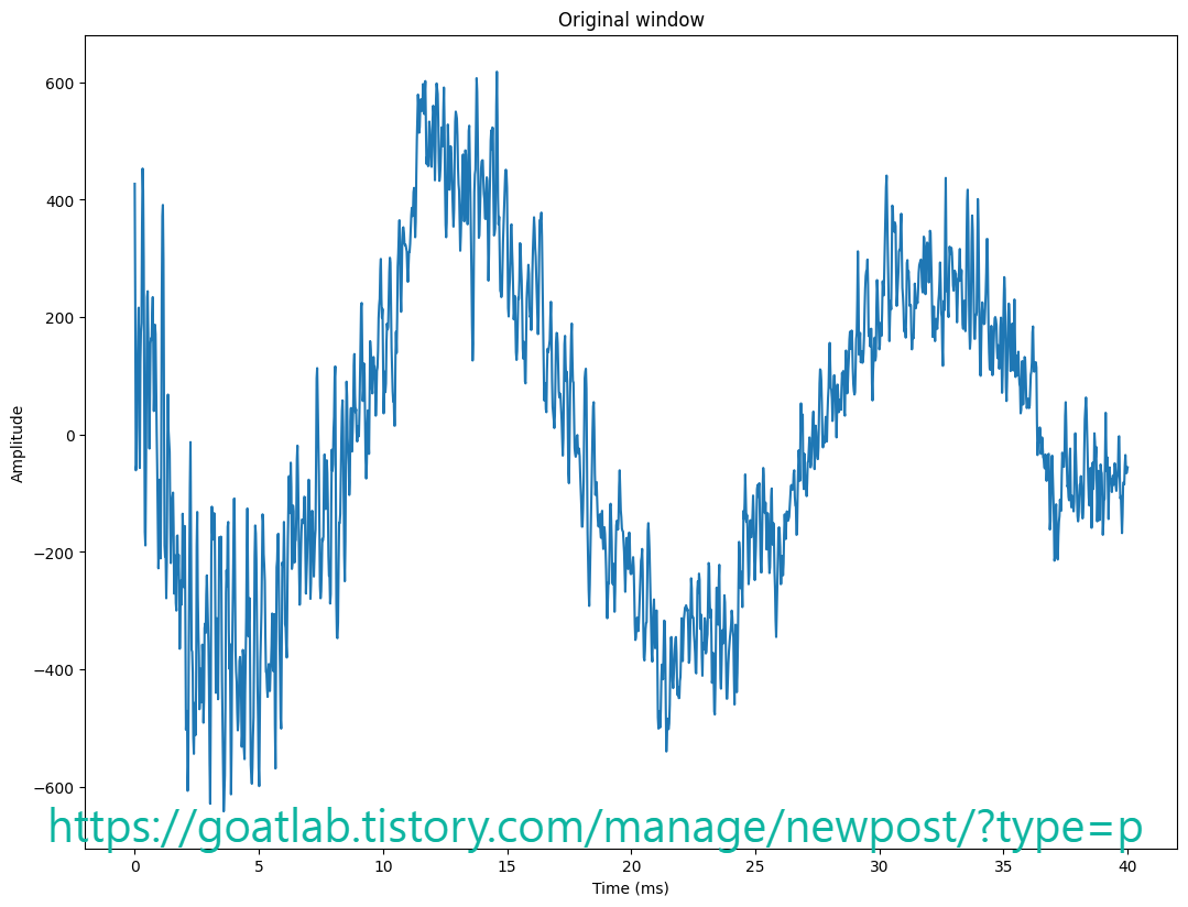
plt.plot(time_vector,data_vector)
plt.title('Original window')
plt.xlabel('Time (ms)')
plt.ylabel('Amplitude')
plt.subplot(322)
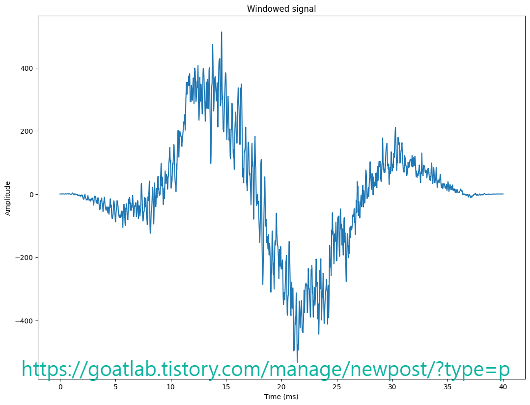
plt.plot(time_vector,window)
plt.title('Windowed signal')
plt.xlabel('Time (ms)')
plt.ylabel('Amplitude')
plt.subplot(323)
plt.plot(frequency_vector,logspectrum)
plt.title('Log-magnitude spectrum')
plt.xlabel('Frequency (kHz)')
plt.ylabel('Magnitude $20\log_{10}|X_k|$')
plt.subplot(324)
plt.plot(frequency_vector,logspectrum)
plt.title('Log-magnitude spectrum (zoomed to low frequencies)')
plt.xlabel('Frequency (kHz)')
plt.ylabel('Magnitude $20\log_{10}|X_k|$')
ax = plt.axis()
ax = [0, 4, ax[2], ax[3]]
plt.axis(ax)
plt.subplot(325)
plt.plot(ctime,np.abs(cepstrum))
plt.title('Cepstrum')
plt.xlabel('Quefrency (ms)')
plt.ylabel('Magnitude $|C_k|$')
ax = plt.axis()
ax = [0, 20, ax[2], ax[3]]
plt.axis(ax)
plt.subplot(326)
plt.plot(ctime,np.log(np.abs(cepstrum)))
plt.title('Log-Cepstrum')
plt.xlabel('Quefrency (ms)')
plt.ylabel('Log-Magnitude $\log|C_k|$')
ax = plt.axis()
ax = [0, 20, ax[2], ax[3]]
plt.axis(ax)
plt.tight_layout()
plt.show()
캡스트럼 특징
스펙트럼의 포락선은 평활화 (smoothed)된 버전이므로 캡스트텀의 낮은 부분에 존재해야 한다. 그러나 lowest 계수의 해석은 직관적이지 않다. 또한, 전력 스펙트럼이 0이거나 0에 매우 가까워 로그 스펙트럼이 음의 무한대에 가까워질 수 있다는 문제가 있다. 고립된 0은 포락선에 영향을 미치지 않아야 하지만 로그 영역에서는 매우 큰 음수 값은 캡스트럼에 큰 기여를 한다. 따라서, 캡스트럼은 포락선 모델링에 적합하지 않다.
그러나 F0 주파수는 일반적으로 캡스트럼에서 피크로서 눈에 띄게 나타난다. 이 영역은 시간 영역과 유사하기 때문에 캡스트럼 피크는 원래 시간 신호의 주기 길이와 동일한 주파수 값으로 표시된다.
def stft(data,fs,window_length_ms=30,window_step_ms=20,windowing_function=None):
    window_length = int(window_length_ms*fs/2000)*2
    window_step = int(window_step_ms*fs/1000)
    if windowing_function is None:
        windowing_function = np.sin(np.pi*np.arange(0.5,window_length,1)/window_length)**2

    total_length = len(data)
    window_count = int( (total_length-window_length)/window_step) + 1

    spectrum_length = int((window_length)/2)+1
    spectrogram = np.zeros((window_count,spectrum_length),dtype=complex)

    for k in range(window_count):
        starting_position = k*window_step

        data_vector = data[starting_position:(starting_position+window_length),]
        window_spectrum = scipy.fft.rfft(data_vector*windowing_function,n=window_length)

        spectrogram[k,:] = window_spectrum

    return spectrogram
spectrogram = stft(data,fs,window_length_ms=window_length_ms,window_step_ms=window_step_ms)
window_count = spectrogram.shape[0]
cepstrogram = np.zeros((len(cepstrum),window_count))
for k in range(window_count):
starting_position = k*window_step
data_vector = data[starting_position:(starting_position+window_length),]
window = data_vector*windowing_function
time_vector = np.linspace(0,window_length_ms,window_length)
spectrum = scipy.fft.rfft(window,n=spectrum_length)
frequency_vector = np.linspace(0,fs/2000,len(spectrum))
# downsample to 16kHz (that is, Nyquist frequency is 8kHz, that is, everything about 8kHz can be removed)
idx = np.nonzero(frequency_vector <= 8)
frequency_vector = frequency_vector[idx]
spectrum = spectrum[idx]
logspectrum = 20*np.log10(np.abs(spectrum))
cepstrum = scipy.fft.rfft(logspectrum)
cepstrogram[:,k] = np.abs(cepstrum)
# cepstrogram[:,k] = np.abs(scipy.fft.rfft(20*np.log10(np.abs(spectrogram[k,idx])),axis=1))
# cepstrogram = np.abs(scipy.fft.rfft(20*np.log10(np.abs(spectrogram[:,idx])),axis=1))
black_eps = 1e-1 # minimum value for the log-value in the spectrogram - helps making the background really black
import matplotlib as mpl
default_figsize = mpl.rcParamsDefault['figure.figsize']
mpl.rcParams['figure.figsize'] = [val*2 for val in default_figsize]
mpl.rcParams['figure.figsize'] = [val*2 for val in default_figsize]
plt.imshow(20*np.log10(np.abs(np.transpose(spectrogram))+black_eps),aspect='auto',origin='lower',extent=[0, len(data)/fs,0, fs/2000])
plt.xlabel('Time (s)')
plt.ylabel('Frequency (kHz)')
plt.axis([0, len(data)/fs, 0, 8])
plt.title('Spectrogram zoomed to 8 kHz')
plt.show()
plt.imshow(np.log(np.abs(cepstrogram)+black_eps),aspect='auto',origin='lower',extent=[0, len(data)/fs,0, ctime[-1]])
#plt.imshow(np.log(np.abs(cepstrogram)+black_eps),aspect='auto',origin='lower')
plt.xlabel('Time (s)')
plt.ylabel('Quefrency (ms)')
plt.axis([0, len(data)/fs, 0, 20])
#plt.title('Spectrogram zoomed to 8 kHz')
plt.show()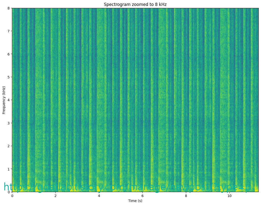
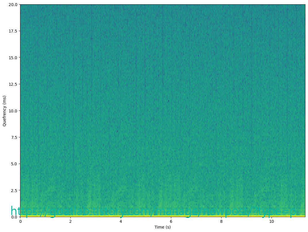
시간이 지남에 따라 곡선이 위아래로 기복이 있는 것을 명확하게 볼 수 있다. quefrency를 주파수로 쉽게 변환할 수 있다 (단, 먼저 밀리초를 초로 변환해야 함).
로그 스펙트럼 다운샘플링
캡스트럼은 포락선와 F0 정보를 추출하는 데는 좋지만, 적은 양의 정보에 많은 수의 계수를 사용한다는 점에서 특별히 효율적이지는 않다. 포락선 정보는 로그 스펙트럼의 천천히 변화하는 모양에 관한 것이므로 간단한 다운샘플링을 통해 추출할 수 있다. 하지만 문제는 전력 스펙트럼은 때때로 임의로 작은 값을 가질 수 있으며, 로그 스펙트럼에서는 거의 무한에 가까운 음의 값으로 변환된다는 것이다. 따라서, 로그 영역의 모든 정보 추출은 음의 무한대에 대한 편향에 취약할 수 있다.
이에 대한 해결책은 전력 스펙트럼에 평활화를 적용하는 것이다. 예를 들어, FIR 필터를 사용하거나 더 일반적으로 삼각형 모양을 사용할 수 있다. 휴리스틱 (heuristic) 용어로는 특정 주파수 주변의 전력의 평균을 구하여 가까운 주파수가 먼 주파수보다 더 큰 가중치를 갖도록 하는 것이다. 그런 다음 가중치 매개변수가 삼각형 모양으로 선택된다. 삼각형 너비의 절반에 해당하는 간격으로 평활화된 샘플을 계산하여 얻은 샘플의 양이 평활화의 양과 일치하도록 한다. 보다 엄격하게는 먼저 FIR 필터를 적용한 다음 적절한 양만큼 다운샘플링을 적용할 수 있지만 최종 결과는 동일하다.
# choose segment from random position in sample
starting_position = np.random.randint(total_length - window_length)

data_vector = data[starting_position:(starting_position+window_length),]
window = data_vector*windowing_function
time_vector = np.linspace(0,window_length_ms,window_length)

spectrum = scipy.fft.rfft(window,n=spectrum_length)
frequency_vector = np.linspace(0,fs/2000,len(spectrum))

# downsample to 16kHz (that is, Nyquist frequency is 8kHz, that is, everything about 8kHz can be removed)
idx = np.nonzero(frequency_vector <= 8)
frequency_vector = frequency_vector[idx]
spectrum = spectrum[idx]

logspectrum = 20*np.log10(np.abs(spectrum))

# filterbank
frequency_step_Hz = 500
frequency_step = int(len(spectrum)*frequency_step_Hz/8000)
frequency_bins = int(len(spectrum)/frequency_step+.5)

slope = np.arange(.5,frequency_step+.5,1)/(frequency_step+1)
backslope = np.flipud(slope)
filterbank = np.zeros((len(spectrum),frequency_bins))
filterbank[0:frequency_step,0] = 1
filterbank[(-frequency_step):-1,-1] = 1

for k in range(frequency_bins-1):
    idx = int((k+0.25)*frequency_step) + np.arange(0,frequency_step)
    filterbank[idx,k+1] = slope
    filterbank[idx,k] = backslope

# smoothing and downsampling
spectrum_smoothed = np.matmul(np.transpose(filterbank),np.abs(spectrum)**2)
logspectrum_smoothed = 10*np.log10(spectrum_smoothed)
frequency_vector_tight = (np.arange(0,frequency_bins,1)+0.25)*frequency_step*8/len(spectrum)

plt.plot(frequency_vector,filterbank)
plt.xlabel('Frequency (kHz)')
plt.ylabel('Amplitude')
plt.title('Triangular filter-bank')
plt.show()

plt.plot(time_vector,data_vector)
plt.title('Original window')
plt.xlabel('Time (ms)')
plt.ylabel('Amplitude')
plt.show()

plt.plot(time_vector,window)
plt.title('Windowed signal')
plt.xlabel('Time (ms)')
plt.ylabel('Amplitude')
plt.show()

plt.plot(frequency_vector,logspectrum,label='Log spectrum')
plt.plot(frequency_vector_tight,logspectrum_smoothed,label='Smoothed')
plt.legend()
plt.title('Log-magnitude spectrum')
plt.xlabel('Frequency (kHz)')
plt.ylabel('Magnitude $20\log_{10}|X_k|$')
plt.show()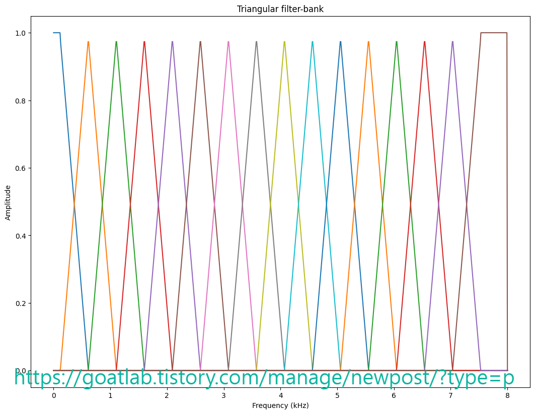
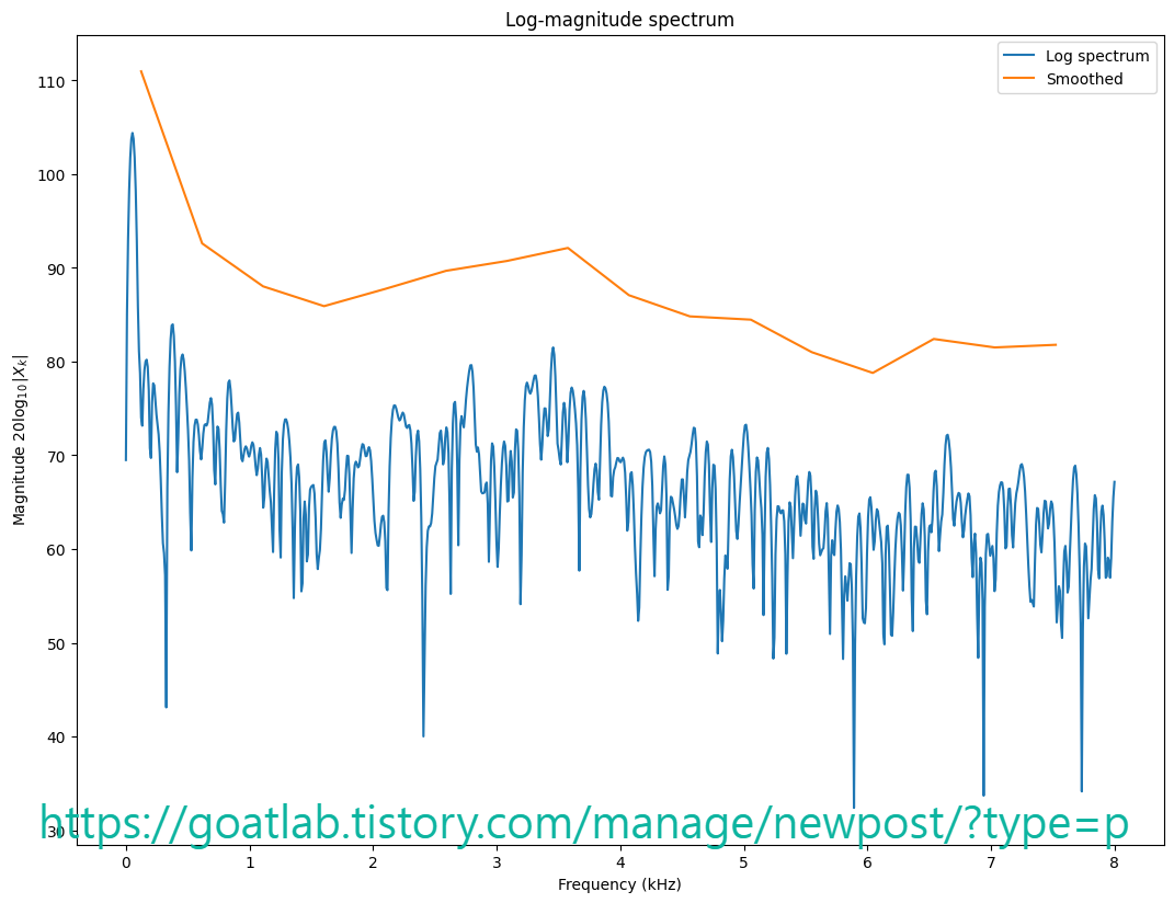
매끄러운 표현은 스펙트럼의 전체 모양, 즉 포락선을 명확하게 포착한다. 이는 낮은 수의 계수로 이를 달성하므로 상당히 효율적인 포락선 모델이다. 그러나 단점은 사람에 대한 특징의 중요성을 반영하지 못한다는 것이다. 로그 변환을 사용하면 크기를 지각 척도에 매핑할 수 있지만, 주파수 척도는 여전히 지각 영역에 매핑되지 않는다.
'Linguistic Intelligence > Audio Processing' 카테고리의 다른 글
| 파형 (Waveform) (0) | 2024.03.27 |
|---|---|
| Mel-Frequency Cepstral Coefficients (MFCC) (0) | 2024.03.20 |
| 오디오 데이터 처리 (2) | 2024.03.06 |
| 소리 및 파형 (0) | 2024.03.06 |
| [Audio Processing] librosa specshow (0) | 2023.07.05 |


