728x90
반응형
SMALL
Python 라이브러리 import
import pandas as pd
import numpy as np
import matplotlib.pylab as plt
import seaborn as sns
import librosa
import librosa.display
import IPython.display as ipd
from glob import glob
from itertools import cycle

sns.set_theme(style="white", palette=None)
color_pal = plt.rcParams["axes.prop_cycle"].by_key()["color"]
color_cycle = cycle(plt.rcParams["axes.prop_cycle"].by_key()["color"])
주파수 (Frequency, Hz)
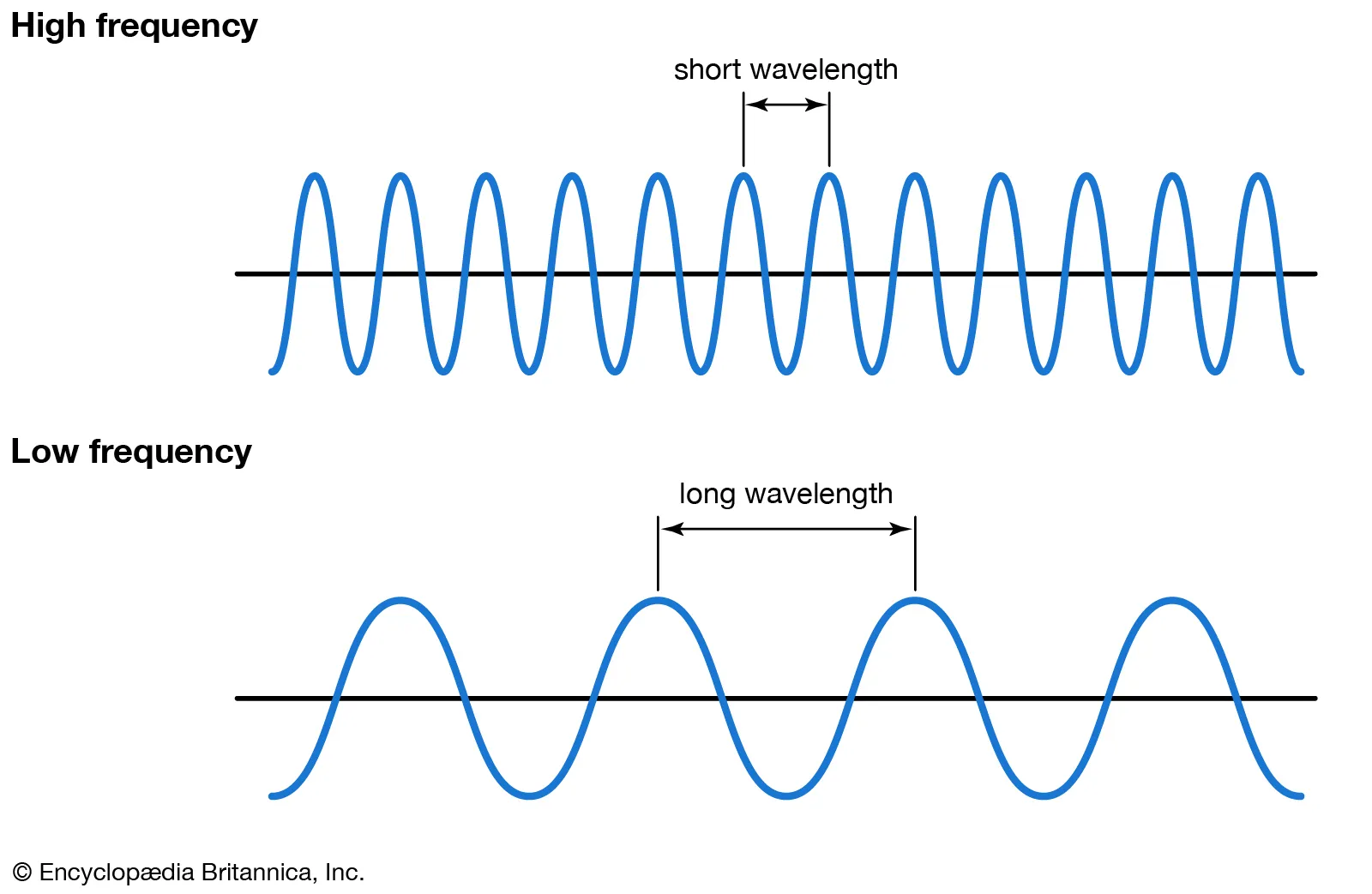
주파수는 파장 (wavelength)의 차이를 설명하며 고음과 저음이 존재한다.
강도 (Intensity, db / power)
강도는 파동의 진폭 (높이)을 나타낸다.
샘플 속도 (Sample Rate)
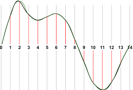
샘플 속도는 컴퓨터가 오디오 파일을 읽는 방식에 따라 다르다. 오디오의 해상도 (resolution)라고 생각하면 된다.
오디오 파일 읽기
오디오 파일에는 mp3, wav, m4a, flac, ogg 등 다양한 유형이 있다. https://samplefocus.com/에서 무료 샘플 파일을 다운 받는다.
audio_files = glob('sample.wav')

# Play audio file
ipd.Audio(audio_files[0])
y, sr = librosa.load(audio_files[0])
print(f'y: {y[:10]}')
print(f'shape y: {y.shape}')
print(f'sr: {sr}')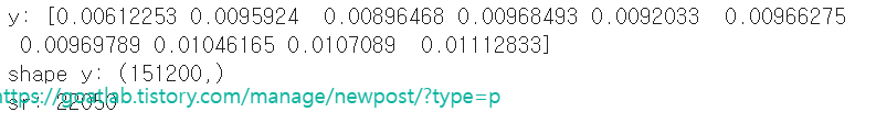
pd.Series(y).plot(figsize=(10, 5),
                  lw=1,
                  title='Raw Audio Example',
                 color=color_pal[0])
plt.show()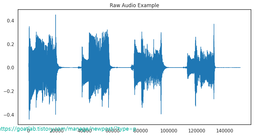
# Trimming leading/lagging silence
y_trimmed, _ = librosa.effects.trim(y, top_db=20)
pd.Series(y_trimmed).plot(figsize=(10, 5),
                  lw=1,
                  title='Raw Audio Trimmed Example',
                 color=color_pal[1])
plt.show()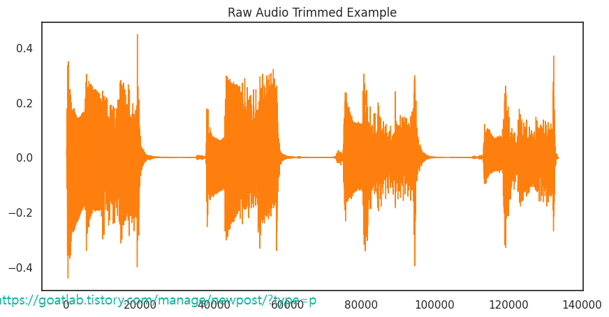
pd.Series(y[30000:30500]).plot(figsize=(10, 5),
                  lw=1,
                  title='Raw Audio Zoomed In Example',
                 color=color_pal[2])
plt.show()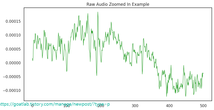
스펙트로그램 (Spectogram)
D = librosa.stft(y)
S_db = librosa.amplitude_to_db(np.abs(D), ref=np.max)
S_db.shape
# Plot the transformed audio data
fig, ax = plt.subplots(figsize=(10, 5))
img = librosa.display.specshow(S_db,
x_axis='time',
y_axis='log',
ax=ax)
ax.set_title('Spectogram Example', fontsize=20)
fig.colorbar(img, ax=ax, format=f'%0.2f')
plt.show()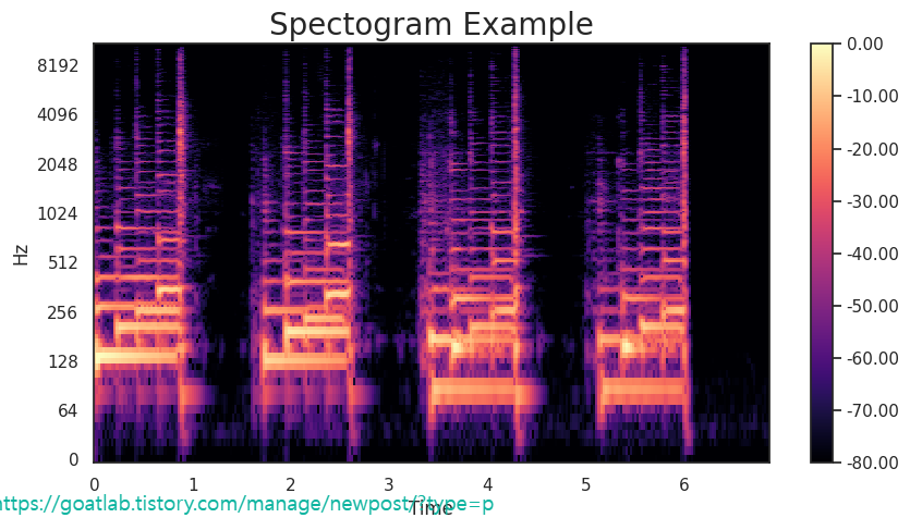
멜 스펙트로그램 (Mel Spectogram)
S = librosa.feature.melspectrogram(y=y,
                                   sr=sr,
                                   n_mels=128 * 2,)
S_db_mel = librosa.amplitude_to_db(S, ref=np.max)
fig, ax = plt.subplots(figsize=(10, 5))
# Plot the mel spectogram
img = librosa.display.specshow(S_db_mel,
                              x_axis='time',
                              y_axis='log',
                              ax=ax)
ax.set_title('Mel Spectogram Example', fontsize=20)
fig.colorbar(img, ax=ax, format=f'%0.2f')
plt.show()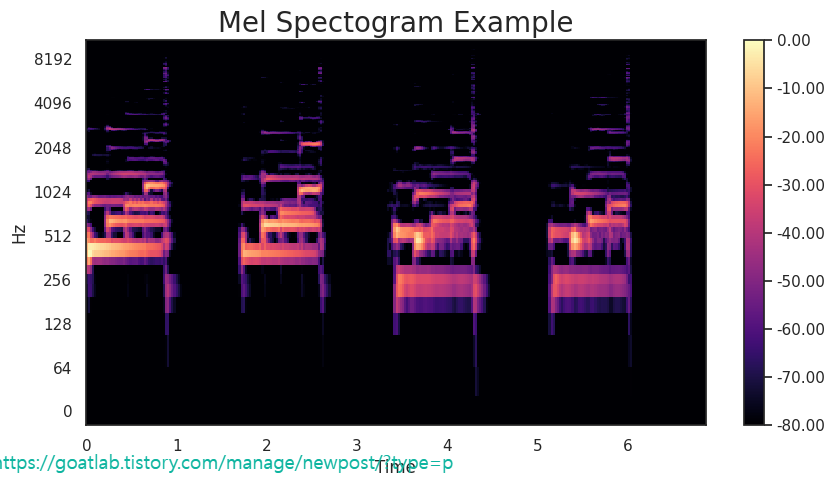
https://www.kaggle.com/code/robikscube/working-with-audio-in-python
🔊 Working with Audio in Python
Explore and run machine learning code with Kaggle Notebooks | Using data from RAVDESS Emotional speech audio
www.kaggle.com
728x90
반응형
LIST
'Linguistic Intelligence > Audio Processing' 카테고리의 다른 글
| Mel-Frequency Cepstral Coefficients (MFCC) (0) | 2024.03.20 |
|---|---|
| 캡스트럼 (Cepstrum) (0) | 2024.03.20 |
| 소리 및 파형 (0) | 2024.03.06 |
| [Audio Processing] librosa specshow (0) | 2023.07.05 |
| [Audio Processing] 시스템 구조 (Systems structures) (0) | 2023.06.15 |


