728x90
반응형
SMALL
동차 좌표
동차 좌표 (Homogenous Coordinate)는 2차원상의 점의 위치를 2차원 벡터가 아닌 3차원 벡터로 표현하는 방법이다.
| - 강체 변환 (rigid transform) : 유클리드 변환(Euclidean transformation)이라고도 불리며, 회전(θ), 이동(t), 두가지 요소만 사용하여 이미지를 변환 - 유사 변환 (similarity transform) : 확대/축소(s), 회전(θ), 이동(t), 세가지 요소를 사용하여 이미지를 변환 |
getRotationMatrix2D(center, angle, scale)
|
주의할 점은 이론적으로는 사영 행렬이 위 식과 같이 3×33×3 행렬이지만, OpenCV에서는 마지막 행을 생략하고 3×23×2 변환행렬을 사용할 수도 있다.
변환 행렬을 실제로 이미지에 적용하여 어파인 변환을 할 때는 warpAffine 함수를 사용한다.
import cv2
import skimage.data

img_astro = skimage.data.astronaut()
img = cv2.cvtColor(img_astro, cv2.COLOR_BGR2GRAY)
rows, cols = img.shape[:2]

# 이미지의 중심점을 기준으로 90도 회전. 크기는 70%
H = cv2.getRotationMatrix2D((cols/2, rows/2), 30, 0.7)

# 50만큼 평행이동
H[:, 2] += 50

H
array([[  0.60621778,   0.35      ,  61.20824764],
       [ -0.35      ,   0.60621778, 240.40824764]])
dst = cv2.warpAffine(img, H, (cols, rows))

fig, [ax1, ax2] = plt.subplots(1, 2, figsize=(13, 13))
ax1.set_title("Original")
ax1.axis("off")
ax1.imshow(img, cmap=plt.cm.gray)
ax2.set_title("Rigid transformed")
ax2.axis("off")
ax2.imshow(dst, cmap=plt.cm.gray)
plt.show()

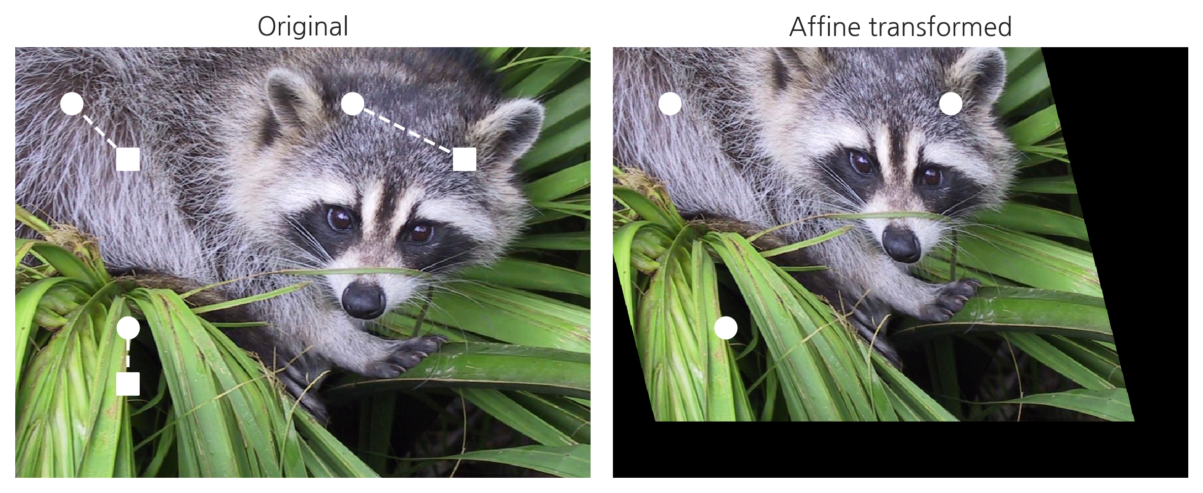
3점 어파인 변환
어파인 변환에 사용되는 행렬을 지정하는데는 3점이 어떻게 변환되는지 알면 된다. OpenCV에는 주어진 두 쌍의 3점으로부터 어파인 변환을 위한 사영행렬을 계산하는 getAffineMatrix 함수를 제공한다.
img = sp.misc.face()
rows, cols, ch = img.shape

pts1 = np.float32([[200, 200], [200, 600], [800, 200]])
pts2 = np.float32([[100, 100], [200, 500], [600, 100]])

pts_x1, pts_y1 = zip(*pts1)
pts_x2, pts_y2 = zip(*pts2)

H_affine = cv2.getAffineTransform(pts1, pts2)
H_affine
array([[ 8.33333333e-01,  2.50000000e-01, -1.16666667e+02],
       [-1.77635684e-17,  1.00000000e+00, -1.00000000e+02]])
img2 = cv2.warpAffine(img, H_affine, (cols, rows))

fig, [ax1, ax2] = plt.subplots(1, 2)

ax1.set_title("Original")
ax1.imshow(img)
ax1.scatter(pts_x1, pts_y1, c='w', s=100, marker="s")
ax1.scatter(pts_x2, pts_y2, c='w', s=100)
ax1.plot(list(zip(*np.stack((pts_x1, pts_x2), axis=-1))),
         list(zip(*np.stack((pts_y1, pts_y2), axis=-1))), "--", c="w")
ax1.axis("off")

ax2.set_title("Affine transformed")
ax2.imshow(img2)
ax2.scatter(pts_x2, pts_y2, c='w', s=100)
ax2.axis("off")

plt.tight_layout()
plt.show()
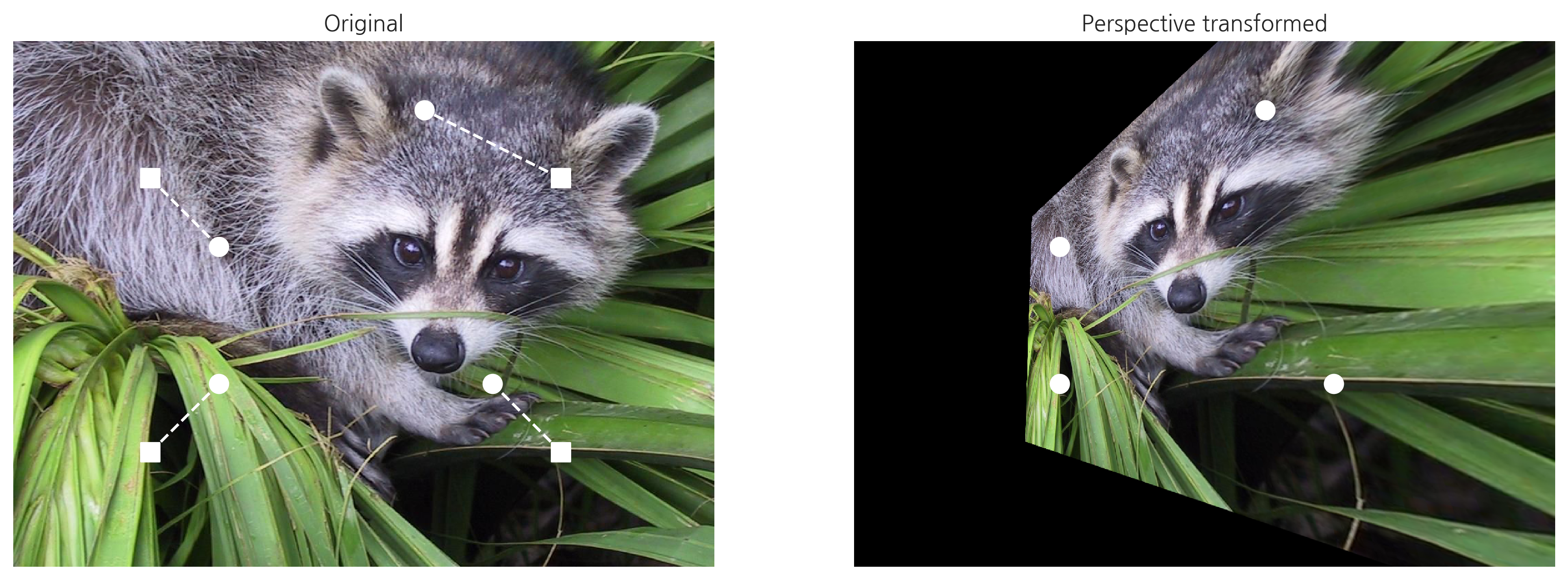
원근 변환
원근변환 (perspective transform)은 핀홀 카메라 (pin-hole camera) 모형을 사용하여 2차원 이미지를 변환하는 방법이다. 원근법 변환은 직선의 성질만 유지가 되고, 선의 평행성은 유지가 되지 않는 변환이다.
원근변환을 지정하는데는 4점이 필요하다. OpenCV에는 주어진 두 쌍의 4점으로부터 원근변환을 위한 사영행렬을 계산하는 getPerspectiveTransform 함수를 제공한다. 실제 변환에는 warpPerspective 함수를 사용한다.
pts1 = np.float32([[200, 200], [200, 600], [800, 200], [800, 600]])
pts2 = np.float32([[300, 300], [300, 500], [600, 100], [700, 500]])

H_perspective = cv2.getPerspectiveTransform(pts1, pts2)
H_perspective
array([[ 3.44169138e-15, -7.62711864e-02,  2.59322034e+02],
       [-3.38983051e-01,  2.79661017e-01,  2.55932203e+02],
       [-6.77966102e-04, -2.54237288e-04,  1.00000000e+00]])
img2 = cv2.warpPerspective(img, H_perspective, (cols, rows))

fig, [ax1, ax2] = plt.subplots(1, 2, figsize=(15, 15))

pts_x, pts_y = zip(*pts1)
pts_x_, pts_y_ = zip(*pts2)

ax1.set_title("Original")
ax1.imshow(img, cmap=plt.cm.bone)
ax1.scatter(pts_x, pts_y, c='w', s=100, marker="s")
ax1.scatter(pts_x_, pts_y_, c='w', s=100)
ax1.plot(list(zip(*np.stack((pts_x, pts_x_), axis=-1))),
         list(zip(*np.stack((pts_y, pts_y_), axis=-1))), "--", c="w")
ax1.axis("off")


ax2.set_title("Perspective transformed")
ax2.imshow(img2, cmap=plt.cm.bone)
ax2.scatter(pts_x_, pts_y_, c='w', s=100)
ax2.axis("off")
plt.show()
이미지 변환 — 데이터 사이언스 스쿨
.ipynb .pdf to have style consistency -->
datascienceschool.net
728x90
반응형
LIST
'AI-driven Methodology > CV (Computer Vision)' 카테고리의 다른 글
| [Computer Vision] paperswithcode (0) | 2022.08.07 |
|---|---|
| [Computer Vision] 임계 처리 (0) | 2022.06.13 |
| [Computer Vision] 컨투어 추정 (0) | 2022.06.13 |
| [Computer Vision] 이미지 컨투어 (0) | 2022.06.13 |
| [Computer Vision] Scikit-Image (0) | 2022.06.13 |


