스마트 워치 PPG 신호 분석
삼성 스마트 워치 장치에서 가져온 원시 PPG 데이터 분석에 HeartPy를 사용하는 방법이다. 측정된 신호는 손목보다 관류 측정이 훨씬 쉬운 손가락 끝이나 귓불의 일반적인 PPG 센서와 비교할 때 훨씬 더 많은 소음을 포함한다.
이러한 신호를 분석하려면 몇 가지 추가 단계가 필요하다.
import numpy as np
import heartpy as hp
import pandas as pd
import matplotlib.pyplot as plt

df = pd.read_csv('raw_ppg.csv')
df.keys()
Index(['ppg', 'timer'], dtype='object')plt.figure(figsize=(12,6))
plt.plot(df['ppg'].values)
plt.show()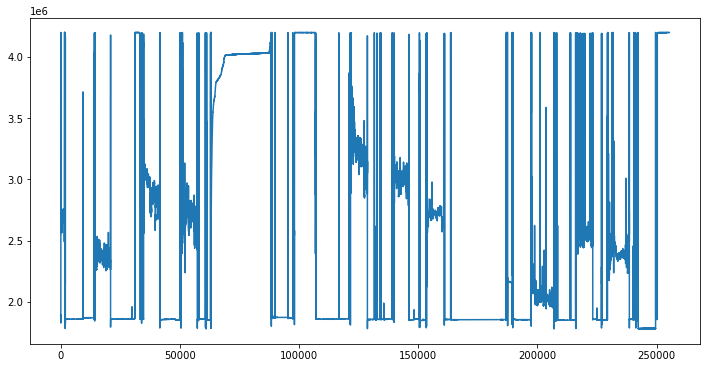
비신호 (센서가 기록하지 않은 기간) 사이에 PPG의 간헐적인 부분이 존재한다. 첫 번째 신호 부분을 자르고 확인한다. 그리고 신호 이외의 섹션을 자동으로 제외하는 방법이 있다.
signal = df['ppg'].values[14500:20500]
timer = df['timer'].values[14500:20500]
plt.plot(signal)
plt.show()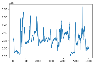
샘플링 속도는 모든 것을 지배하는 하나의 척도이다. 다른 모든 것을 계산하는 데 사용된다. HeartPy에는 타이머 열에서 샘플링 속도를 가져오는 여러 가지 방법이 있다. 타이머 열의 형식을 살펴보고 현재 작업 중인 내용을 살펴 본다.
timer[0:20]array(['11:10:57.978', '11:10:58.078', '11:10:58.178', '11:10:58.279',
'11:10:58.379', '11:10:58.479', '11:10:58.579', '11:10:58.679',
'11:10:58.779', '11:10:58.879', '11:10:58.980', '11:10:59.092',
'11:10:59.180', '11:10:59.283', '11:10:59.381', '11:10:59.481',
'11:10:59.582', '11:10:59.681', '11:10:59.781', '11:10:59.882'],
dtype=object)
형식은 'hours:minutes:seconds.miliseconds'이다. HeartPy는 get_samplate_datetime이라는 날짜 문자열과 시간 문자열로 작동할 수 있는 datetime 함수와 함께 제공된다. 도움말에서 작동 방식을 확인하면 된다.
help(hp.get_samplerate_datetime)Help on function get_samplerate_datetime in module heartpy.datautils:
get_samplerate_datetime(datetimedata, timeformat='%H:%M:%S.%f')
determine sample rate based on datetime
Function to determine sample rate of data from datetime-based timer
list or array.
Parameters
----------
timerdata : 1-d numpy array or list
sequence containing datetime strings
timeformat : string
the format of the datetime-strings in datetimedata
default : '%H:%M:%S.f' (24-hour based time including ms: e.g. 21:43:12.569)
Returns
-------
out : float
the sample rate as determined from the timer sequence provided
Examples
--------
We load the data like before
>>> data, timer = load_exampledata(example = 2)
>>> timer[0]
'2016-11-24 13:58:58.081000'
Note that we need to specify the timeformat used so that datetime understands
what it's working with:
>>> round(get_samplerate_datetime(timer, timeformat = '%Y-%m-%d %H:%M:%S.%f'), 3)
100.42# Seems easy enough, right? Now let's determine the sample rate
sample_rate = hp.get_samplerate_datetime(timer, timeformat = '%H:%M:%S.%f')
print('sampling rate is: %.3f Hz' %sample_rate)sampling rate is: 9.986 Hz
샘플링 비율은 꽤 낮지만 전력을 절약하기 위해 많은 스마트 시계와 함께 작동한다. BPM을 결정하는 데 있어 이것은 괜찮지만, 어떤 심박변이도 (HRV) 측정도 매우 정확하지는 않을 것이다. 하지만, 필요에 따라 그것은 괜찮을 수도 있다.
샘플링 속도와 관련된 두 번째 고려 사항은 안정적인지 여부이다. 스마트 시계를 포함한 많은 기기들은 한 번에 많은 일을 한다. 심박수를 측정하는 것 외에 다른 작업을 하는 OS를 실행하므로, 10Hz로 측정할 때 OS는 100ms마다 정확하게 측정할 준비가 되지 않을 수 있다. 따라서, 샘플링 속도는 달라질 수 있다. 이것을 시각화한다.
from datetime import datetime

# let's create a list 'newtimer' to house our datetime objects
newtimer = [datetime.strptime(x, '%H:%M:%S.%f') for x in timer]

# let's compute the real distances from entry to entry
elapsed = []
for i in range(len(newtimer) - 1):
    elapsed.append(1 / ((newtimer[i+1] - newtimer[i]).microseconds / 1000000))

# and plot the results
plt.figure(figsize=(12,4))
plt.plot(elapsed)
plt.xlabel('Sample number')
plt.ylabel('Actual sampling rate in Hz')
plt.show()

print('mean sampling rate: %.3f' %np.mean(elapsed))
print('median sampling rate: %.3f'%np.median(elapsed))
print('standard deviation: %.3f'%np.std(elapsed))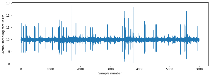
mean sampling rate: 9.987
median sampling rate: 10.000
standard deviation: 0.183
신호 평균은 10Hz에 가깝고 분산이 낮다. 12Hz로 산발적인 피크 또는 9Hz로 하강하는 것은 타이머의 부정확성을 나타내지만 드물게 발생한다. 목적상 이것은 현재로썬 괜찮지만 물론, 정확한 샘플링 속도를 갖도록 신호를 보간하고 다시 샘플링할 수 있지만 계산된 측정값에 미치는 영향은 미미할 수 있다.
# Let's plot 4 minutes of the segment we selected to get a view
# of what we're working with
plt.figure(figsize=(12,6))
plt.plot(signal[0:int(240 * sample_rate)])
plt.title('original signal')
plt.show()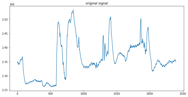
가장 먼저 주목해야 할 것은 진폭이 확연히 달라진다는 점이다. 대역 통과 필터로 돌려서 심박수가 아닌 주파수를 모두 빼내야 한다. 0.7Hz (42BPM) 미만과 3.5Hz (210BPM) 이상의 주파수를 뺀다.
# Let's run it through a standard butterworth bandpass implementation to remove everything < 0.8 and > 3.5 Hz.
filtered = hp.filter_signal(signal, [0.7, 3.5], sample_rate=sample_rate,
                            order=3, filtertype='bandpass')

# let's plot first 240 seconds and work with that!
plt.figure(figsize=(12,12))
plt.subplot(211)
plt.plot(signal[0:int(240 * sample_rate)])
plt.title('original signal')
plt.subplot(212)
plt.plot(filtered[0:int(240 * sample_rate)])
plt.title('filtered signal')
plt.show()

plt.figure(figsize=(12,6))
plt.plot(filtered[0:int(sample_rate * 60)])
plt.title('60 second segment of filtered signal')
plt.show()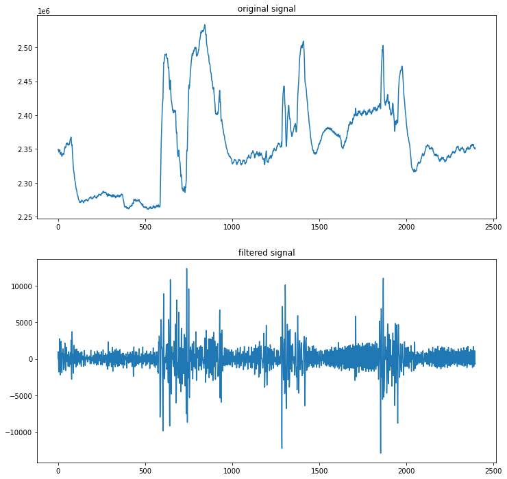
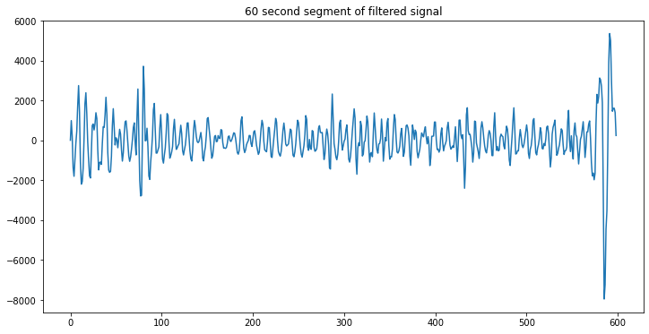
여전히 낮은 품질이지만 적어도 심장 박동수는 이제 꽤 보인다.
GitHub - paulvangentcom/heartrate_analysis_python: Python Heart Rate Analysis Package, for both PPG and ECG signals
Python Heart Rate Analysis Package, for both PPG and ECG signals - GitHub - paulvangentcom/heartrate_analysis_python: Python Heart Rate Analysis Package, for both PPG and ECG signals
github.com
'Python Library > HeartPy' 카테고리의 다른 글
| [HeartPy] 스마트 링 PPG 신호 분석 (0) | 2022.08.24 |
|---|---|
| [HeartPy] 스마트 워치 PPG 신호 분석 (2) (0) | 2022.08.24 |
| [HeartPy] ECG 신호 분석 (0) | 2022.08.24 |
| [HeartPy] PPG 신호 분석 (0) | 2022.08.24 |
| [HeartPy] 심박수 분석 (Heart Rate Analysis) (0) | 2022.08.23 |


