Baseline Correction
EEG는 시간 분해 신호이므로 실험 질문과 관련이 없는 일시적인 드리프트가 있는 경우가 많다. 다양한 내부 및 외부 소스로 인해 시간이 지남에 따라 그리고 전극 간에도 변화하는 일시적인 드리프트가 발생할 수 있다. 이러한 드리프트의 영향을 줄이기 위해 소위 베이스라인 보정을 수행하는 것이 일반적이다. 기본적으로 이것은 기준 기간 동안, 즉 외부 사건이 발생하기 전의 EEG 활동을 사용하여 자극 후 간격 (즉, 외부 사건이 발생한 후 시간)에 걸쳐 활동을 수정하는 것으로 구성된다. 기준선 보정을 위한 다양한 접근 방식이 있다. 전통적인 방법은 기준선과 자극 후 간격의 모든 시점에서 기준선 기간의 평균을 빼는 것이다.
Baseline Correction with MNE
MNE에서 기준선 보정을 적용하려면 epochs 객체의 apply_baseline() 함수에 매개변수로 시간 간격을 전달해야 한다. 시간 간격으로 'None'을 지정하면 기준선 보정이 적용되지 않는다. 모든 시간 간격에 기준선 보정을 적용하려면 (None, None)을 사용해야 한다. 이 함수는 기준선 수정된 epochs 개체를 반환하고 개체도 수정한다.
# For elimiating warnings
from warnings import simplefilter
simplefilter(action='ignore', category=FutureWarning)

import mne
import mne.viz
import numpy as np
%matplotlib inline

#Load epoched data
data_file = '../datasets/904_1_PDDys_ODDBALL_Clean_curated.fif'
# Read the EEG epochs:
epochs = mne.read_epochs(data_file, verbose='error')

# Plot of initial evoked object
epochs.average().plot()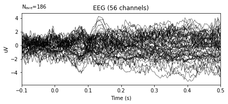
초기 신호는 기준선 보정에 의해 수정된다. 초기 epoch 객체를 변경 없이 유지하려면 apply_baseline() 함수를 호출하기 전에 다른 변수에 복사해야 한다. 그렇지 않으면 손실된다. Python에서는 원본 객체가 수정될 때 얕은 복사본을 수정할 수 있다. 그러나 깊은 복사본은 원본 개체와 독립적이다. 따라서 우리의 경우 epochs 객체의 깊은 복사본이 필요하다.
Selecting baseline interval
일반적으로 기준선 간격은 우리의 예에서 자극 시작 시간 간격에 대한 자극으로 선택된다. 이 간격은 자극의 시작인 -100ms에서 0ms이다.
import copy
epochs_wo_bc = copy.deepcopy(epochs)
# baseline correction
inteval = (-0.1, 0)
bc_epochs = epochs.apply_baseline(inteval)

# Plot of baseline-corrected evoked signal
bc_epochs.average().plot()
#Modified evoked object
epochs.average().plot()
epochs_wo_bc.average().plot()
위의 예에서 주어진 신호의 진폭 편차가 크게 감소했다.
또는 아래 플롯에서와 같이 단일 시도와 평균을 보여주는 플롯을 통해 유사한 관찰을 수행할 수 있다. 이 플롯에서 검은색 선은 평균을 나타내고 나머지는 단일 시도이다.
이 플롯은 Python의 Matplotlib 라이브러리를 사용하여 그려진다.
from matplotlib import pyplot as plt
%matplotlib inline

def plotChannel(ch_index, with_baselineCorrection, without_baselineCorrection):

    ch = ch_index
    data_types = ['original', 'bc']

    for i in range(len(data_types)):

        fig, ax = plt.subplots(figsize=(20, 10))
        ax.set_xlabel('Time instances')
        ax.set_ylabel('Volt')
        #plt.ylim(-1.1, 1.5)
        if data_types[i] == 'bc':
            plt.title('Plot of Single Trials with Baseline Correction')
            for i in range(len(with_baselineCorrection.get_data())):
                ax.plot(with_baselineCorrection.times, with_baselineCorrection.get_data()[i,ch,:])
            ax.plot(with_baselineCorrection.average().times, with_baselineCorrection.average().data[ch,:], color='black', label='Average of Trials')

        else:
            plt.title('Plot of Single Trials without Baseline Correction')
            for i in range(len(without_baselineCorrection.get_data())):
                ax.plot(without_baselineCorrection.times, without_baselineCorrection.get_data()[i,ch,:])
            ax.plot(without_baselineCorrection.average().times, without_baselineCorrection.average().data[ch,:], color='black', label='Average of Trials')

        legend = ax.legend(loc='upper center', shadow=True, fontsize='large')
        plt.show()
ch_index = 5
plotChannel(ch_index, bc_epochs, epochs_wo_bc)
Manual Baseline Correction
MNE에서 기준선 보정이 가능하지만 라이브러리나 패키지에 의존하지 않고 수동으로 쉽게 적용할 수 있다.
epochs_for_bc = copy.deepcopy(epochs_wo_bc)
먼저 기준 계산을 위한 시간 간격을 선택한다. 각 에포크에 대해 선택한 시간 간격의 평균을 계산한다. 그렇게 함으로써 데이터 세트의 각 에포크에 대한 기준 값을 갖게 된다.
time_interval = [-0.1, 0]
interval_baseline = [i for i in epochs_for_bc.times if i >= time_interval[0] and i <= time_interval[1]]
baseline = []
data = epochs_for_bc.get_data()
for e in range(data.shape[0]):
    avg_epoch = np.mean(data[e,:,:len(interval_baseline)], axis=1)
    baseline.append(avg_epoch)
baseline = np.asarray(baseline)
베이스라인 수정의 마지막 단계는 에포크 데이터에서 각 에포크에 대해 계산된 베이스라인 값을 빼는 것이다.
for e in range(len(epochs_for_bc.get_data())):
    for i in range(len(epochs_for_bc.ch_names)):
        epochs_for_bc.get_data()[e,i,:] = epochs_for_bc.get_data()[e,i,:] - baseline[e,i]
기준선 수정을 적용하기 전후에 채널 3을 플로팅한다.
plotChannel(ch_index, epochs_for_bc, epochs_wo_bc)
수동 기준선 계산이 올바른지 확인하려면 mne 및 수동 기준선 수정 모두에 기준선 수정을 적용하기 전에 아래 예와 같이 에포크를 선택하고 에포크 데이터에서 기준선 수정된 에포크 데이터를 뺀다. 결과적으로 두 접근 방식 모두에 대한 기준 값의 배열을 얻게 된다. 마지막으로 기준 값을 비교한다. 모든 기준 값이 동일하면 계산이 정확하다는 결론을 내릴 수 있다.
manual_baseline_values = np.subtract(epochs_wo_bc._data[1,:,:], epochs_for_bc._data[1,:,:])
mne_baseline_values = np.subtract(epochs_wo_bc._data[1,:,:], bc_epochs._data[1,:,:])

if manual_baseline_values.all() == mne_baseline_values.all():
    print('Baseline values calculated manually and via MNE are the same !!!')
else:
    print('Baseline values are different !!!')
Baseline values calculated manually and via MNE are the same !!!
MNE는 데이터에서 기준선 간격의 평균을 빼는 방식으로 apply_baseline 함수를 제공한다. 따라서 수동 기준선 수정에 대해 동일한 방법을 따른다. 그러나 기준선 수정을 위해 개발된 다른 접근 방식이 있다는 점은 주목할 가치가 있다.
https://neuro.inf.unibe.ch/AlgorithmsNeuroscience/Tutorial_files/BaselineCorrection.html
Baseline Correction
Baseline Correction Tutorial #3: Baseline Correction As EEG is a time-resolving signal, it may often have temporal drifts which are unrelated to o...
neuro.inf.unibe.ch
'Brain Engineering > MNE' 카테고리의 다른 글
| Machine Learning : Formatting a dataset (0) | 2022.04.05 |
|---|---|
| Preprocessing : Choosing a Reference (0) | 2022.04.05 |
| Preprocessing : Data Visualization (0) | 2022.04.05 |
| Preprocessing : Data Loading (2) (0) | 2022.04.05 |
| Preprocessing : Data Loading (1) (0) | 2022.04.05 |


