728x90
반응형
SMALL
데이터 전처리
import tensorflow as tf
import numpy as np
import matplotlib.pyplot as plt
from tensorflow.keras.layers import SimpleRNN, LSTM, Dense
from tensorflow.keras import Sequential

# data 생성
x = np.arange(0, 100, 0.1)
y = 0.5*np.sin(2*x) - np.cos(x/2.0)

seq_data = y.reshape(-1,1)

print(seq_data.shape)
print(seq_data[:5])
(1000, 1)
[[-1. ]
[-0.89941559]
[-0.80029499]
[-0.70644984]
[-0.62138853]]plt.grid()
plt.title('0.5*sin(2x)-cos(x/2)')
plt.xlabel('time')
plt.ylabel('amplitude')
plt.plot(seq_data)
plt.show()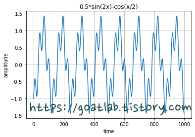
def seq2dataset(seq, window, horizon):
    X = []
    Y = []

    for i in range(len(seq)-(window+horizon)+1):
        x = seq[i:(i+window)]
        y = (seq[i+window+horizon-1])

        X.append(x)
        Y.append(y)

    return np.array(X), np.array(Y)

w = 20  # window size
h = 1  # horizon factor

X, Y = seq2dataset(seq_data, w, h)

print(X.shape, Y.shape)
(980, 20, 1) (980, 1)split_ratio = 0.8
split = int(split_ratio*len(X))
x_train = X[0:split]
y_train = Y[0:split]
x_test = X[split:]
y_test = Y[split:]
print(x_train.shape, y_train.shape, x_test.shape, y_test.shape)(784, 20, 1) (784, 1) (196, 20, 1) (196, 1)
모델 생성
model = Sequential()

model.add(SimpleRNN(units=128, activation='tanh', input_shape=x_train[0].shape))

model.add(Dense(1))

model.summary()
Model: "sequential"
_________________________________________________________________
Layer (type) Output Shape Param #
=================================================================
simple_rnn (SimpleRNN) (None, 128) 16640
dense (Dense) (None, 1) 129
=================================================================
Total params: 16,769
Trainable params: 16,769
Non-trainable params: 0
_________________________________________________________________from datetime import datetime
model.compile(loss='mse', optimizer='adam', metrics=['mae'])
start_time = datetime.now()
hist = model.fit(x_train, y_train,
epochs=100,
validation_data=(x_test, y_test))
end_time = datetime.now()
print('Elapsed Time => ', end_time-start_time)plt.title('Loss Trend')
plt.plot(hist.history['loss'], label='loss')
plt.plot(hist.history['val_loss'], label='val_loss')
plt.xlabel('epoch')
plt.ylabel('loss')
plt.grid()
plt.legend(loc='best')
plt.show()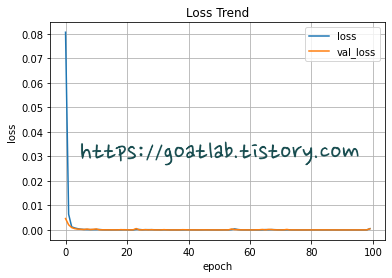
pred = model.predict(x_test)

print(pred.shape)
7/7 [==============================] - 0s 4ms/step
(196, 1)rand_idx = np.random.randint(0, len(y_test), size=5)
print('random idx = ',rand_idx, '\n')
print('pred = ', pred.flatten()[rand_idx])
print('label = ', y_test.flatten()[rand_idx])
rand_idx = np.random.randint(0, len(y_test), size=5)
print('\n\nrandom idx = ',rand_idx, '\n')
print('pred = ', pred.flatten()[rand_idx])
print('label = ', y_test.flatten()[rand_idx])random idx = [ 9 152 148 25 84]
pred = [ 0.6421721 1.0176921 1.3699332 1.1660998 -0.4494172]
label = [ 0.6363903 0.99169316 1.36121199 1.14384382 -0.41652189]
random idx = [152 181 100 75 14]
pred = [ 1.0176921 -0.13476941 -0.8855729 -1.1017574 1.1269114 ]
label = [ 0.99169316 -0.12930711 -0.83954079 -1.06389327 1.11572477]plt.plot(pred, label='prediction')
plt.plot(y_test, label='label')
plt.grid()
plt.legend(loc='best')
plt.show()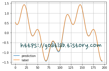
728x90
반응형
LIST
'AI-driven Methodology > ANN' 카테고리의 다른 글
| [ANN] GRU으로 삼성전자 주가 예측 (0) | 2022.10.21 |
|---|---|
| [ANN] LSTM으로 삼성전자 주가 예측 (0) | 2022.10.21 |
| [ANN] SimpleRNN (1) (0) | 2022.10.19 |
| [ANN] LSTM (Long-Short Term Memory) (0) | 2022.10.11 |
| [ANN] 심층 신경망 (Deep Neural Network) (0) | 2022.10.11 |


