Epoching continuous data
객체와 이벤트 배열은 클래스 생성자로 생성하는 객체 Raw를 생성하는 데 필요한 최소한의 것이다. 여기에서 몇 가지 데이터 품질 제약 조건도 지정한다. 피크 대 피크 신호 진폭이 해당 채널 유형에 대한 합리적인 한계를 초과하는 모든 에포크를 거부한다. 이것은 거부 사전을 사용하여 수행된다. 데이터에 있는 모든 채널 유형에 대한 임계값을 포함하거나 생략할 수 있다. 여기에 제공된 값은 이 특정 데이터 세트에 적합하지만 다른 하드웨어 또는 기록 조건에 맞게 조정해야 할 수도 있다.
reject_criteria = dict(mag=4000e-15,     # 4000 fT
                       grad=4000e-13,    # 4000 fT/cm
                       eeg=150e-6,       # 150 µV
                       eog=250e-6)       # 250 µV
또한 이벤트 사전을 event_id 매개변수로 전달하고 (정수 이벤트 ID 대신 풀링하기 쉬운 이벤트 레이블로 작업할 수 있도록) tmin및 tmax (각 에포크를 시작하고 종료하는 각 이벤트에 상대적인 시간)를 지정한다. 기본적 Raw으로 Epochs 데이터는 메모리에 로드되지 않지만 (필요할 때만 디스크에서 액세스됨) preload=True에서는 거부 기준의 결과를 볼 수 있도록 매개변수 를 사용하여 메모리에 강제로 로드한다.
epochs = mne.Epochs(raw, events, event_id=event_dict, tmin=-0.2, tmax=0.5,
                    reject=reject_criteria, preload=True)
---
Not setting metadata
319 matching events found
Setting baseline interval to [-0.19979521315838786, 0.0] sec
Applying baseline correction (mode: mean)
Created an SSP operator (subspace dimension = 4)
4 projection items activated
Using data from preloaded Raw for 319 events and 106 original time points ...
    Rejecting  epoch based on EOG : ['EOG 061']
    Rejecting  epoch based on EOG : ['EOG 061']
    Rejecting  epoch based on MAG : ['MEG 1711']
    Rejecting  epoch based on EOG : ['EOG 061']
    Rejecting  epoch based on EOG : ['EOG 061']
    Rejecting  epoch based on MAG : ['MEG 1711']
    Rejecting  epoch based on EEG : ['EEG 008']
    Rejecting  epoch based on EOG : ['EOG 061']
    Rejecting  epoch based on EOG : ['EOG 061']
    Rejecting  epoch based on EOG : ['EOG 061']
10 bad epochs dropped
청각적 반응과 시각적 반응을 비교할 수 있도록 왼쪽 / 오른쪽 자극 프리젠테이션에 걸쳐 풀링할 것이다. 신호가 왼쪽이나 오른쪽으로 치우치는 것을 방지하기 위해 equalize_event_counts 먼저 각 조건에서 epoch를 무작위로 샘플링하여 가장 적은 좋은 epoch를 가진 조건에 존재하는 epoch 수와 일치시킨다.
conds_we_care_about = ['auditory/left', 'auditory/right',
                       'visual/left', 'visual/right']
epochs.equalize_event_counts(conds_we_care_about)  # this operates in-place
aud_epochs = epochs['auditory']
vis_epochs = epochs['visual']
del raw, epochs  # free up memory

Out : Dropped 7 epochs: 121, 195, 258, 271, 273, 274, 275
개체와 마찬가지로 Raw 개체 Epochs에도 여러 가지 기본 제공 플로팅 방법이 있다. 하나는 plot_image각 에포크를 신호 크기를 나타내는 색상과 함께 이미지 맵의 한 행으로 표시하는 것이다. 평균 유발 반응과 센서 위치가 이미지 아래에 표시된다.
aud_epochs.plot_image(picks=['MEG 1332', 'EEG 021'])
Not setting metadata
136 matching events found
No baseline correction applied
0 projection items activated
0 bad epochs dropped
Not setting metadata
136 matching events found
No baseline correction applied
0 projection items activated
0 bad epochs dropped
Time-frequency analysis
mne.time_frequency 서브모듈은 시간-주파수 표현, 전력 스펙트럼 밀도 및 교차 스펙트럼 밀도를 계산하는 여러 알고리즘의 구현을 제공한다 . 예를 들어, 여기에서 Morlet 웨이블릿을 사용하여 다양한 주파수와 시간에서 유도 전력을 청각 에포크에 대해 계산한다. 이 데이터 세트에서 결과는 특히 유익하지 않다 (단지 "청각 N100" 응답을 불러일으킴).
frequencies = np.arange(7, 30, 3)
power = mne.time_frequency.tfr_morlet(aud_epochs, n_cycles=2, return_itc=False,
                                      freqs=frequencies, decim=3)
power.plot(['MEG 1332'])
Removing projector <Projection | PCA-v1, active : True, n_channels : 102>
Removing projector <Projection | PCA-v2, active : True, n_channels : 102>
Removing projector <Projection | PCA-v3, active : True, n_channels : 102>
Removing projector <Projection | Average EEG reference, active : True, n_channels : 60>
No baseline correction applied
Estimating evoked responses
aud_epochs및 vis_epochs에 있으므로 각 조건에서 epoch를 함께 평균화하여 청각 대 시각적 자극에 대한 유발된 반응의 추정치를 얻을 수 있다. average이것은 객체에 대한 메서드를 호출 Epochs한 다음 모듈의 함수를 사용하여 두 객체 mne.viz의 각 센서 유형에 대한 전역 필드 전력을 비교하는 것처럼 간단하다.
aud_evoked = aud_epochs.average()
vis_evoked = vis_epochs.average()

mne.viz.plot_compare_evokeds(dict(auditory=aud_evoked, visual=vis_evoked),
                             legend='upper left', show_sensors='upper right')
Multiple channel types selected, returning one figure per type.
combining channels using "gfp"
combining channels using "gfp"
combining channels using "gfp"
combining channels using "gfp"
combining channels using "gfp"
combining channels using "gfp"
Evoked와 같은 다른 플로팅 방법을 사용하여 각 객체를 더 자세히 볼 수도 있다 . 여기에서 EEG 채널만 검사하고 등전두 전극에 대한 고전적인 청각 유발 N100-P200 패턴을 확인한 다음 임의의 추가 시간에 두피 지형을 플로팅한다.
aud_evoked.plot_joint(picks='eeg')
aud_evoked.plot_topomap(times=[0., 0.08, 0.1, 0.12, 0.2], ch_type='eeg')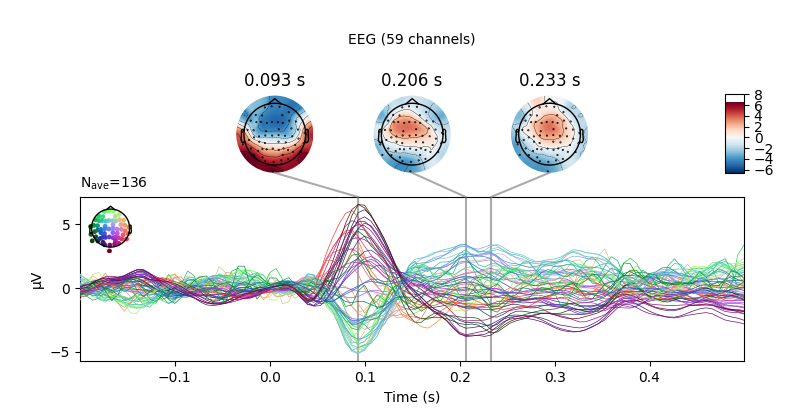
Projections have already been applied. Setting proj attribute to True.
Removing projector <Projection | PCA-v1, active : True, n_channels : 102>
Removing projector <Projection | PCA-v2, active : True, n_channels : 102>
Removing projector <Projection | PCA-v3, active : True, n_channels : 102>
이 기능을 사용하여 유발된 객체를 결합하여 조건 간의 대비를 표시할 수도 있다. mne.combine_evoked를 전달하여 간단한 차이를 생성할 수 있다 . 그런 다음 다음을 사용하여 각 센서의 차이 파동을 플로팅한다.
evoked_diff = mne.combine_evoked([aud_evoked, vis_evoked], weights=[1, -1])
evoked_diff.pick_types(meg='mag').plot_topo(color='r', legend=False)
Removing projector <Projection | Average EEG reference, active : True, n_channels : 60>
Inverse modeling
센서 데이터를 이 피험자의 소스 공간 (구조적 MRI 스캔에 의해 추정된 피질 표면 또는 피질 부피 내의 포인트 세트)에 투영함으로써 유발된 활동의 기원을 추정할 수 있다 . MNE-Python은 이를 수행하는 많은 방법 (동적 통계적 매개변수 매핑, 쌍극자 피팅, 빔 형성기 등)을 지원한다. 여기서 최소 표준 추정 (MNE)을 사용하여 피질 표면에 제한된 활성화의 연속 맵을 생성한다. MNE는 선형 역 연산자를 사용하여 EEG+MEG 센서 측정값을 소스 공간에 투영한다. 역 연산자는 주제에 대한 순방향 솔루션 과 센서 측정의 공분산 추정값에서 계산된다.
# load inverse operator
inverse_operator_file = os.path.join(sample_data_folder, 'MEG', 'sample',
                                     'sample_audvis-meg-oct-6-meg-inv.fif')
inv_operator = mne.minimum_norm.read_inverse_operator(inverse_operator_file)
# set signal-to-noise ratio (SNR) to compute regularization parameter (λ²)
snr = 3.
lambda2 = 1. / snr ** 2
# generate the source time course (STC)
stc = mne.minimum_norm.apply_inverse(vis_evoked, inv_operator,
                                     lambda2=lambda2,
                                     method='MNE')  # or dSPM, sLORETA, eLORETA
---
Reading inverse operator decomposition from /home/circleci/mne_data/MNE-sample-data/MEG/sample/sample_audvis-meg-oct-6-meg-inv.fif...
    Reading inverse operator info...
    [done]
    Reading inverse operator decomposition...
    [done]
    305 x 305 full covariance (kind = 1) found.
    Read a total of 4 projection items:
        PCA-v1 (1 x 10²) active
        PCA-v2 (1 x 10²) active
        PCA-v3 (1 x 10²) active
        Average EEG reference (1 x 60) active
    Noise covariance matrix read.
    22494 x 22494 diagonal covariance (kind = 2) found.
    Source covariance matrix read.
    22494 x 22494 diagonal covariance (kind = 6) found.
    Orientation priors read.
    22494 x 22494 diagonal covariance (kind = 5) found.
    Depth priors read.
    Did not find the desired covariance matrix (kind = 3)
    Reading a source space...
    Computing patch statistics...
    Patch information added...
    Distance information added...
    [done]
    Reading a source space...
    Computing patch statistics...
    Patch information added...
    Distance information added...
    [done]
    2 source spaces read
    Read a total of 4 projection items:
        PCA-v1 (1 x 10²) active
        PCA-v2 (1 x 10²) active
        PCA-v3 (1 x 10²) active
        Average EEG reference (1 x 60) active
    Source spaces transformed to the inverse solution coordinate frame
Preparing the inverse operator for use...
    Scaled noise and source covariance from nave = 1 to nave = 136
    Created the regularized inverter
    Created an SSP operator (subspace dimension = 3)
    Created the whitener using a noise covariance matrix with rank 302 (3 small eigenvalues omitted)
Applying inverse operator to "0.50 × visual/left + 0.50 × visual/right"...
    Picked 305 channels from the data
    Computing inverse...
    Eigenleads need to be weighted ...
    Computing residual...
    Explained  70.2% variance
    Combining the current components...
[done]
대상의 피질 표면에 소스 추정치를 표시하려면 샘플 대상의 구조적 MRI 파일 (the subjects_dir)에 대한 경로도 필요하다.
# path to subjects' MRI files
subjects_dir = os.path.join(sample_data_folder, 'subjects')
# plot the STC
stc.plot(initial_time=0.1, hemi='split', views=['lat', 'med'],
         subjects_dir=subjects_dir)
Overview of MEG/EEG analysis with MNE-Python — MNE 1.0.0 documentation
Overview of MEG/EEG analysis with MNE-Python This tutorial covers the basic EEG/MEG pipeline for event-related analysis: loading data, epoching, averaging, plotting, and estimating cortical activity from sensor data. It introduces the core MNE-Python data
mne.tools
'Brain Engineering > MNE Python' 카테고리의 다른 글
| [MNE-Python] 원시 데이터에서 이벤트 구문 분석 (2) (0) | 2022.03.23 |
|---|---|
| [MNE-Python] 원시 데이터에서 이벤트 구문 분석 (1) (0) | 2022.03.23 |
| [MNE-Python] 내부 데이터 수정 (0) | 2022.03.22 |
| [MNE-Python] MEG / EEG analysis (1) (0) | 2022.03.18 |
| MNE (0) | 2022.03.14 |


